spark下线性模型 spark.mllib

我还是参考官方的文档来写这个部分，顺便梳理下原理，给出对应代码及运行结果，一点也不复杂。

数学公式

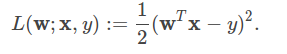
许多的机器学习的算法实际上可以被写成凸优化的问题，比如说寻找凸函数$f$的极小值，它取决于权重向量ｗ，那么我们可以将优化目标函数写成：

这里$x_i \in R^d$是训练数据，$y_i \in R$是它们对应的标签，线性方法可以表示成$L(w;x,y)$，有几类mllib中的分类和回归算法都可以归为这一类。
目标函数由两个部分，正则项，控制模型的复杂度，以及loss（亏损函数），它评估训练数据的模型误差。

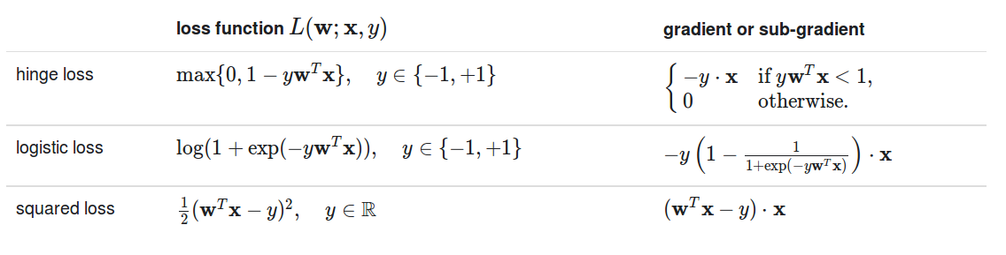
Loss functions

mllib中支持的亏损函数和它们的梯度(对ｗ)为：

正则项

正则项鼓励简单的模型，避免overfitting.

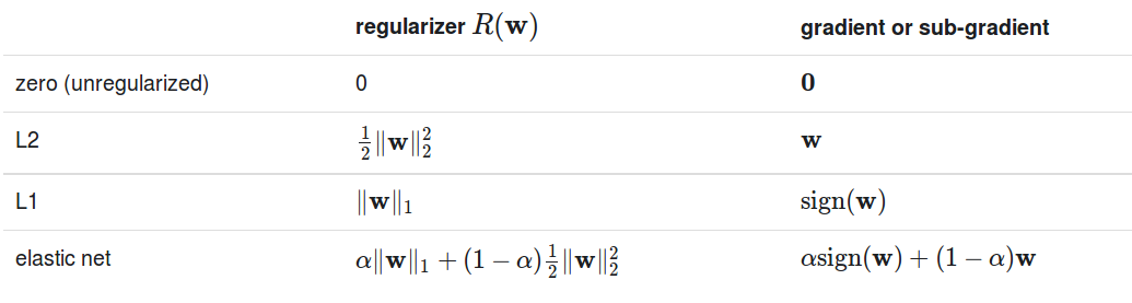
L2约束一般来说比Ｌ1约束更平滑，然而，Ｌ１约束可以帮助提升权重项的稀疏性，因此可以获得更小的容易解释的模型，在特征选择方面非常有用。Elastic网是Ｌ1和L2的结合。

优化

使用凸优化的方法来对目标函数进行优化，spark.mllib使用两种方法，分别是SGD和Ｌ-BFGS，我们在优化这一章来进一部解释。目前，大多数算法的ＡＰＩｓ支持随机梯度下降算法SGD，少数支持Ｌ-BFGS算法。

分类

常见的有二分类的问题，将样本分为正样本和负样本，超过两类就是多分类问题。
在spark.mllib中，支持两种线性分类方法，分别是SVMs以及逻辑回归。线性SVMs的方法仅仅支持二分类，逻辑回归同时还支持多分类的问题。对于两种方法，spark.mllib都支持Ｌ1和Ｌ２的规则项。
训练集用MLlib中的LabeledPoint的RDD来表示,所有的标签都是从０开始的，需要注意的是，在二分类问题的数学表示中，负样本写成-1, 然而这里我们把负样本写成０．

线性SVM

损失函数定义为：

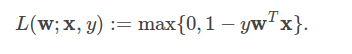
默认情况下，线性ＳＶＭ使用的是L2约束，当然同时也可以使用L1约束，这种情况下它就变成线性规划问题。
这是我在Intellij下运行通过的scala版本的代码，可读性非常高。

import org.apache.spark.{SparkContext, SparkConf}
import org.apache.spark.mllib.classification.{SVMModel, SVMWithSGD}
import org.apache.spark.mllib.evaluation.BinaryClassificationMetrics
import org.apache.spark.mllib.util.MLUtils

object testSVM{

  def main(args:Array[String]): Unit ={


    val conf = new SparkConf()
      .setMaster("local[2]")
      .setAppName("testSVM")
    var sc = new SparkContext(conf)

    // Load training data in LIBSVM format.
    val data = MLUtils.loadLibSVMFile(sc, "/home/hadoop/spark/data/mllib/sample_libsvm_data.txt")

    // Split data into training (60%) and test (40%).
    val splits = data.randomSplit(Array(0.6, 0.4), seed = 11L)
    val training = splits(0).cache()
    val test = splits(1)

    // Run training algorithm to build the model
    val numIterations = 100
    val model = SVMWithSGD.train(training, numIterations)

    // Clear the default threshold.
    model.clearThreshold()

    // Compute raw scores on the test set.
    val scoreAndLabels = test.map { point =>
      val score = model.predict(point.features)
      (score, point.label)
    }

    // Get evaluation metrics.
    val metrics = new BinaryClassificationMetrics(scoreAndLabels)
    val auROC = metrics.areaUnderROC()

    println("Area under ROC = " + auROC)

    // Save and load model
    model.save(sc, "myModelPath")
    val sameModel = SVMModel.load(sc, "myModelPath")

  }

}

运行可以得到结果为：
Area under ROC = 1.0
注意输入的格式为：
label index1:value1 index2:value2 …
它是稀疏的

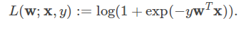
逻辑回归

逻辑回归中的损失函数可以表示成：

对于二分类问题，算法输出一个二值的逻辑回归模型，给定一个数据点，表示成ｘ，通过运用逻辑函数

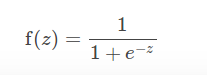
表示，其中$z=W^Tx$, 如果$f(z)>0.5$那么输出就为正，样本为正样本，否则为负，样本为负样本。
二值逻辑回归也可以推广到多模态，用于多分类问题。比如说有Ｋ个可能的输出，其中一个输出作为pivot，其余的Ｋ-1个用于与之区分。在spark.mllib中，第一个class 0 作为pivot类。
多分类的问题由Ｋ-1个二值的逻辑回归组成，给定一个新的数据点，我们将运行K-１个模型，拥有最大的概率的类将被选为预测的类。
我们实现两个算法来求解逻辑回归问题：　一个是mini-batch的梯度下降算法，一个是L-BFGS算法。我们推荐使用L-BFGS。

/**
  * Created by hadoop on 16-2-16.
  */
import org.apache.spark.{SparkConf, SparkContext}
import org.apache.spark.mllib.classification.{LogisticRegressionWithLBFGS, LogisticRegressionModel}
import org.apache.spark.mllib.evaluation.MulticlassMetrics
import org.apache.spark.mllib.regression.LabeledPoint
import org.apache.spark.mllib.linalg.Vectors
import org.apache.spark.mllib.util.MLUtils
object testLR {
  def main(args:Array[String]): Unit = {
    val conf = new SparkConf()
      .setMaster("local[2]")
      .setAppName("testSVM")
    var sc = new SparkContext(conf)
    // Load training data in LIBSVM format.
    val data = MLUtils.loadLibSVMFile(sc, "/home/hadoop/spark/data/mllib/sample_libsvm_data.txt")

    // Split data into training (60%) and test (40%).
    val splits = data.randomSplit(Array(0.6, 0.4), seed = 11L)
    val training = splits(0).cache()
    val test = splits(1)

    // Run training algorithm to build the model
    val model = new LogisticRegressionWithLBFGS()
      .setNumClasses(10)
      .run(training)

    // Compute raw scores on the test set.
    val predictionAndLabels = test.map { case LabeledPoint(label, features) =>
      val prediction = model.predict(features)
      (prediction, label)
    }

    // Get evaluation metrics.
    val metrics = new MulticlassMetrics(predictionAndLabels)
    val precision = metrics.precision
    println("Precision = " + precision)

    // Save and load model
    model.save(sc, "myModelPath")
    val sameModel = LogisticRegressionModel.load(sc, "myModelPath")
  }
}

输出为：
Precision = 1.0

Regression

Linear least squares, Lasso, and ridge regression

linear least squares是回归问题中最常见的构造，损失函数可以写成

可以使用不同类型的规则项，比如说ordinary least squares 或者linear least squares 它们没有使用规则项，
ridge regression使用L2规则项，Lasso使用的L1规则项。对于所有的模型，平均损失以及训练误差为

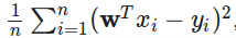
也就是平均squared error。
下面的例子，首先载入数据，解析成LabeledPoint的RDD格式，随后使用LinearRegressionWithSGD来构造一个简单的线性model来预测值。用squared error来表示拟合情况。

import org.apache.spark.{SparkContext, SparkConf}
import org.apache.spark.mllib.regression.LabeledPoint
import org.apache.spark.mllib.regression.LinearRegressionModel
import org.apache.spark.mllib.regression.LinearRegressionWithSGD
import org.apache.spark.mllib.linalg.Vectors
object Regression {
  def main(args:Array[String]): Unit ={
    val conf = new SparkConf()
      .setMaster("local[2]")
      .setAppName("testSVM")
    var sc = new SparkContext(conf)

    // Load and parse the data
    val data = sc.textFile("/home/hadoop/spark/data/mllib/ridge-data/lpsa.data")
    val parsedData = data.map { line =>
      val parts = line.split(',')
      LabeledPoint(parts(0).toDouble, Vectors.dense(parts(1).split(' ').map(_.toDouble)))
    }.cache()

    // Building the model
    val numIterations = 100
    val model = LinearRegressionWithSGD.train(parsedData, numIterations)

    // Evaluate model on training examples and compute training error
    val valuesAndPreds = parsedData.map { point =>
      val prediction = model.predict(point.features)
      (point.label, prediction)
    }
    val MSE = valuesAndPreds.map{case(v, p) => math.pow((v - p), 2)}.mean()
    println("training Mean Squared Error = " + MSE)

    // Save and load model
    model.save(sc, "myModelPath")
    val sameModel = LinearRegressionModel.load(sc, "myModelPath")
  }
}

输出结果为：
training Mean Squared Error = 6.207597210613578

注意其中的，创建dense vector的方法

// Create a dense vector (1.0, 0.0, 3.0).
val dv: Vector = Vectors.dense(1.0, 0.0, 3.0)
// Create a sparse vector (1.0, 0.0, 3.0) by specifying its indices and values corresponding to nonzero entries.
val sv1: Vector = Vectors.sparse(3, Array(0, 2), Array(1.0, 3.0))
// Create a sparse vector (1.0, 0.0, 3.0) by specifying its nonzero entries.
val sv2: Vector = Vectors.sparse(3, Seq((0, 1.0), (2, 3.0))) //第一项为向量的长度

Streaming linear regression

当数据按照流的方式到来时，采用在线回归模型的方式是很好的，目前mllib支持streaming 线性回归。这个拟合和离线的方式差不多，只是每来一批数据，就拟合一次，所以可以不断的更新。

开发者实现

mllib实现了一个简单的分布式的SGD，基于原始的梯度下降，算法的规则项为regParam，以及不同的参数用于随机梯度下降(stepSize, numIterations, miniBatchFraction)。对于每一项，都支持三种可能的规则项（none,L1,L2）
For Logistic Regression, L-BFGS version is implemented under LogisticRegressionWithLBFGS, and this version supports both binary and multinomial Logistic Regression while SGD version only supports binary Logistic Regression. However, L-BFGS version doesn’t support L1 regularization but SGD one supports L1 regularization. When L1 regularization is not required, L-BFGS version is strongly recommended since it converges faster and more accurately compared to SGD by approximating the inverse Hessian matrix using quasi-Newton method.

Algorithms are all implemented in Scala:

SVMWithSGD
LogisticRegressionWithLBFGS
LogisticRegressionWithSGD
LinearRegressionWithSGD
RidgeRegressionWithSGD
LassoWithSGD

---

参考文献
http://spark.apache.org/docs/latest/mllib-linear-methods.html