


Interacting with Contrastive Language-Image Pre-Training (CLIP) model on AMD GPU — ROCm Blogs

2024年4月16日,由Sean Song撰写.
引言
对比语言-图像预训练(CLIP)是一种多模态深度学习模型,连接视觉和自然语言。它在OpenAI的论文“通过自然语言监督学习可转移的视觉模型” (2021) 中被介绍,并在大量(4亿)网页抓取的数据图像-字幕对上进行了对比训练(这是最早进行此类训练的模型之一)。
在预训练阶段,CLIP被训练去预测批次中图像和文本之间的语义关联。这包括确定哪些图像-文本对彼此之间最相关或最密切。这一过程涉及图像编码器和文本编码器的同时训练。其目标是最大化批次中图像和文本对嵌入间的余弦相似度,同时最小化错误对嵌入之间的相似度。通过这种方式,该模型学习到一个多模态的嵌入空间。对这些相似度分数使用对称交叉熵损失进行优化。

图片来源: 通过自然语言监督学习可转移的视觉模型.
In the subsequent sections of the blog, we will leverage the PyTorch framework along 在随后的博客部分,我们将利用*PyTorch*框架与*ROCm*一起运行CLIP模型,以计算任意图像和文本输入之间的相似度。
设置
此演示使用以下设置创建。有关全面的支持详情,请参阅ROCm 文档。
-
硬件和操作系统:
-
Ubuntu 22.04.3 LTS
-
软件:
任意图像和文本输入之间的相似度计算
步骤1:入门
首先,确认GPU的可用性。
!rocm-smi --showproductname
========== ROCm System Management Interface =========================
==================== Product Info ===================================
    GPU[0]      : Card series:      AMD INSTINCT MI250 (MCM) OAM AC MBA
    GPU[0]      : Card model:       0x0b0c
    GPU[0]      : Card vendor:      Advanced Micro Devices, Inc. [AMD/ATI]
    GPU[0]      : Card SKU:         D65209
    ====================================================================================
====================== End of ROCm SMI Log ================================
接下来,安装CLIP和所需的库。
! pip install git+https://github.com/openai/CLIP.git ftfy regex tqdm matplotlib
步骤2:加载模型
import torch
import clip
import numpy as np

# 在这个博客中我们将加载 ViT-L/14@336px 的 CLIP 模型
model, preprocess = clip.load("ViT-L/14@336px")
model.cuda().eval()
# 检查模型架构
print(model)
# 检查预处理器
print(preprocess)
输出:
    CLIP(
  (visual): VisionTransformer(
    (conv1): Conv2d(3, 1024, kernel_size=(14, 14), stride=(14, 14), bias=False)
    (ln_pre): LayerNorm((1024,), eps=1e-05, elementwise_affine=True)
    (transformer): Transformer(
      (resblocks): Sequential(
        (0): ResidualAttentionBlock(
          (attn): MultiheadAttention(
            (out_proj): NonDynamicallyQuantizableLinear(in_features=1024, out_features=1024, bias=True)
          )
          (ln_1): LayerNorm((1024,), eps=1e-05, elementwise_affine=True)
          (mlp): Sequential(
            (c_fc): Linear(in_features=1024, out_features=4096, bias=True)
            (gelu): QuickGELU()
            (c_proj): Linear(in_features=4096, out_features=1024, bias=True)
          )
          (ln_2): LayerNorm((1024,), eps=1e-05, elementwise_affine=True)
        )
        (1): ResidualAttentionBlock(
          (attn): MultiheadAttention(
            (out_proj): NonDynamicallyQuantizableLinear(in_features=1024, out_features=1024, bias=True)
          )
          (ln_1): LayerNorm((1024,), eps=1e-05, elementwise_affine=True)
          (mlp): Sequential(
            (c_fc): Linear(in_features=1024, out_features=4096, bias=True)
            (gelu): QuickGELU()
            (c_proj): Linear(in_features=4096, out_features=1024, bias=True)
          )
          (ln_2): LayerNorm((1024,), eps=1e-05, elementwise_affine=True)
        )
        ...
        (23): ResidualAttentionBlock(
          (attn): MultiheadAttention(
            (out_proj): NonDynamicallyQuantizableLinear(in_features=1024, out_features=1024, bias=True)
          )
          (ln_1): LayerNorm((1024,), eps=1e-05, elementwise_affine=True)
          (mlp): Sequential(
            (c_fc): Linear(in_features=1024, out_features=4096, bias=True)
            (gelu): QuickGELU()
            (c_proj): Linear(in_features=4096, out_features=1024, bias=True)
          )
          (ln_2): LayerNorm((1024,), eps=1e-05, elementwise_affine=True)
        )
      )
    )
    (ln_post): LayerNorm((1024,), eps=1e-05, elementwise_affine=True)
  )
  (transformer): Transformer(
    (resblocks): Sequential(
      (0): ResidualAttentionBlock(
        (attn): MultiheadAttention(
          (out_proj): NonDynamicallyQuantizableLinear(in_features=768, out_features=768, bias=True)
        )
        (ln_1): LayerNorm((768,), eps=1e-05, elementwise_affine=True)
        (mlp): Sequential(
          (c_fc): Linear(in_features=768, out_features=3072, bias=True)
          (gelu): QuickGELU()
          (c_proj): Linear(in_features=3072, out_features=768, bias=True)
        )
        (ln_2): LayerNorm((768,), eps=1e-05, elementwise_affine=True)
      )
      (1): ResidualAttentionBlock(
        (attn): MultiheadAttention(
          (out_proj): NonDynamicallyQuantizableLinear(in_features=768, out_features=768, bias=True)
        )
        (ln_1): LayerNorm((768,), eps=1e-05, elementwise_affine=True)
        (mlp): Sequential(
          (c_fc): Linear(in_features=768, out_features=3072, bias=True)
          (gelu): QuickGELU()
          (c_proj): Linear(in_features=3072, out_features=768, bias=True)
        )
        (ln_2): LayerNorm((768,), eps=1e-05, elementwise_affine=True)
      )
      ...
      (11): ResidualAttentionBlock(
        (attn): MultiheadAttention(
          (out_proj): NonDynamicallyQuantizableLinear(in_features=768, out_features=768, bias=True)
        )
        (ln_1): LayerNorm((768,), eps=1e-05, elementwise_affine=True)
        (mlp): Sequential(
          (c_fc): Linear(in_features=768, out_features=3072, bias=True)
          (gelu): QuickGELU()
          (c_proj): Linear(in_features=3072, out_features=768, bias=True)
        )
        (ln_2): LayerNorm((768,), eps=1e-05, elementwise_affine=True)
      )
    )
  )
  (token_embedding): Embedding(49408, 768)
  (ln_final): LayerNorm((768,), eps=1e-05, elementwise_affine=True)
)


Compose(
    Resize(size=336, interpolation=bicubic, max_size=None, antialias=warn)
    CenterCrop(size=(336, 336))
    <function _convert_image_to_rgb at 0x7f8616295630>
    ToTensor()
    Normalize(mean=(0.48145466, 0.4578275, 0.40821073), std=(0.26862954, 0.26130258, 0.27577711))
)
步骤3:检查图像和文本
我们从 COCO 数据集 中获取 8 张示例图片及其文本描述,并将图片特征和文本特征进行比对,计算相似度。
import os
import matplotlib.pyplot as plt
from PIL import Image

# 使用来自 COCO 数据集的图像及其文本描述
image_urls  = [
    "http://farm1.staticflickr.com/6/8378612_34ab6787ae_z.jpg",
    "http://farm9.staticflickr.com/8456/8033451486_aa38ee006c_z.jpg",
    "http://farm9.staticflickr.com/8344/8221561363_a6042ba9e0_z.jpg",
    "http://farm5.staticflickr.com/4147/5210232105_b22d909ab7_z.jpg",
    "http://farm4.staticflickr.com/3098/2852057907_29f1f35ff7_z.jpg",
    "http://farm4.staticflickr.com/3324/3289158186_155a301760_z.jpg",
    "http://farm4.staticflickr.com/3718/9148767840_a30c2c7dcb_z.jpg",
    "http://farm9.staticflickr.com/8030/7989105762_4ef9e7a03c_z.jpg"
]

text_descriptions = [
    "a cat standing on a wooden floor",
    "an airplane on the runway",
    "a white truck parked next to trees",
    "an elephant standing in a zoo",
    "a laptop on a desk beside a window",
    "a giraffe standing in a dirt field",
    "a bus stopped at a bus stop",
    "two bunches of bananas in the market"
]
显示八张图片及其对应的文本描述。
import requests
from io import BytesIO

images_for_display=[]
images=[]

# 创建一个新图形
plt.figure(figsize=(12, 6))
size = (400, 320)
# 依次遍历每个 URL 并在子图中绘制图像
for i, url1 in enumerate(image_urls):
    # # 从 URL 获取图像
    response = requests.get(url1)
    image = Image.open(BytesIO(response.content))
    image = image.resize(size)

    # 添加子图 (2 行,4 列,索引为 i+1)
    plt.subplot(2, 4, i + 1)

    # 绘制图像
    plt.imshow(image)
    plt.axis('off')  # Turn off axes labels

    # 添加标题(可选)
    plt.title(f'{text_descriptions[i]}')

    images_for_display.append(image)
    images.append(preprocess(image))

# 调整布局以防止重叠
plt.tight_layout()

# 显示图
plt.show()

第 4 步:生成特征
接下来,我们准备图像和文本输入,并继续执行模型的前向传播。这一步将分别提取图像和文本特征。
image_inputs = torch.tensor(np.stack(images)).cuda()
text_tokens = clip.tokenize(["It is " + text for text in text_descriptions]).cuda()

with torch.no_grad():
    image_features = model.encode_image(image_inputs).float()
    text_features = model.encode_text(text_tokens).float()
步骤5:计算文本与图像之间的相似度得分
我们对特征进行归一化,并计算每对的点积。
image_features /= image_features.norm(dim=-1, keepdim=True)
text_features /= text_features.norm(dim=-1, keepdim=True)
similarity_score = text_features.cpu().numpy() @ image_features.cpu().numpy().T
步骤6:可视化文本与图像之间的相似度
def plot_similarity(text_descriptions, similarity_score, images_for_display):
    count = len(text_descriptions)
    fig, ax = plt.subplots(figsize=(18, 15))
    im = ax.imshow(similarity_score, cmap=plt.cm.YlOrRd)
    plt.colorbar(im, ax=ax)

    # y轴刻度:文本描述
    ax.set_yticks(np.arange(count))
    ax.set_yticklabels(text_descriptions, fontsize=12)
    ax.set_xticklabels([])
    ax.xaxis.set_visible(False)

    for i, image in enumerate(images_for_display):
        ax.imshow(image, extent=(i - 0.5, i + 0.5, -1.6, -0.6), origin="lower")


    for x in range(similarity_score.shape[1]):
        for y in range(similarity_score.shape[0]):
            ax.text(x, y, f"{similarity_score[y, x]:.2f}", ha="center", va="center", size=10)

    ax.spines[["left", "top", "right", "bottom"]].set_visible(False)

    # 设置x轴和y轴的限制
    ax.set_xlim([-0.5, count - 0.5])
    ax.set_ylim([count + 0.5, -2])

    # 为图表添加标题
    ax.set_title("Text and Image Similarity Score calculated with CLIP", size=14)

    plt.show()

plot_similarity(text_descriptions, similarity_score, images_for_display)
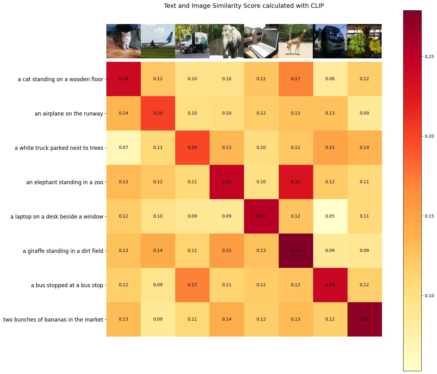
如论文所述,CLIP的目标是在批次内最大化图像和文本对的嵌入相似度,同时最小化错误对的嵌入相似度。在结果中可以观察到,对角线上的单元格在各自的列和行中表现出最高的值。


 被折叠的 条评论
为什么被折叠?
被折叠的 条评论
为什么被折叠?
 到【灌水乐园】发言


