


- 梯度下降法
由于LR的损失函数为:
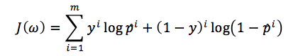
这样就变成了求min(Jω)
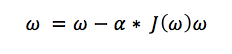
其中α为步长,直到Jω不能再小时停止
梯度下降法的最大问题就是会陷入局部最优,并且每次在对当前样本计算cost的时候都需要去遍历全部样本才能得到cost值,这样计算速度就会慢很多(虽然在计算的时候可以转为矩阵乘法去更新整个ω值)
- 随机梯度下降法
现在好多框架(mahout)中一般使用随机梯度下降法,它在计算cost的时候只计算当前的代价,最终cost是在全部样本迭代一遍之求和得出,还有他在更新当前的参数w的时候并不是依次遍历样本,而是从所有的样本中随机选择一条进行计算,它方法收敛速度快(一般是使用最大迭代次数),并且还可以避免局部最优,并且还很容易并行(使用参数服务器的方式进行并行)
![]()
这里SGD可以改进的地方就是使用动态的步长
![]()
- 其他优化方法
- 拟牛顿法(使用Hessian矩阵和cholesky分解)
- BFGS
- L-BFGS
优缺点:无需选择学习率α,更快,但是更复杂。
Matlab实现:
https://github.com/fairlyxu/ml/tree/master/mlclass-ex2-007/mlclass-ex2-007/mlclass-ex2
| function [J, grad] = costFunction(theta, X, y) %COSTFUNCTION Compute cost and gradient for logistic regression % J = COSTFUNCTION(theta, X, y) computes the cost of using theta as the % parameter for logistic regression and the gradient of the cost % w.r.t. to the parameters.
% Initialize some useful values m = length(y); % number of training examples
% You need to return the following variables correctly J = 0; grad = zeros(size(theta));
% ====================== YOUR CODE HERE ====================== % Instructions: Compute the cost of a particular choice of theta. % You should set J to the cost. % Compute the partial derivatives and set grad to the partial % derivatives of the cost w.r.t. each parameter in theta % % Note: grad should have the same dimensions as theta % for i=1:m J= J- y(i,:)*log(sigmoid(X(i,:)*theta))-(1-y(i,:))*log(1-sigmoid(X(i,:)*theta)); grad(1) = grad(1) + (sigmoid(X(i,:) * theta) - y(i)) * X(i,1); grad(2) = grad(2) + (sigmoid(X(i,:) * theta) - y(i)) * X(i,2); grad(3) = grad(3) + (sigmoid(X(i,:) * theta) - y(i)) * X(i,3);
end grad = grad /m J = J/m; %grad = X' * (sigmoid(X * theta) - y) / m %grad = grad/m;
% ============================================================= end
grad = zeros(3); for i = 1:m grad(1) = grad(1) + (sigmoid(X(i,:) * theta) - y(i)) * X(i,1); grad(2) = grad(2) + (sigmoid(X(i,:) * theta) - y(i)) * X(i,2); grad(3) = grad(3) + (sigmoid(X(i,:) * theta) - y(i)) * X(i,3); end grad = grad /m
|


 1万+
1万+


 被折叠的 条评论
为什么被折叠?
被折叠的 条评论
为什么被折叠?
 到【灌水乐园】发言


