梯度提升机（Gradient Boosting Machine）之 LightGBM

最新推荐文章于 2023-09-19 21:21:46 发布

FlameAlpha

最新推荐文章于 2023-09-19 21:21:46 发布

阅读量1.2w

点赞数 53

分类专栏：机器学习 # 机器学习算法补充文章标签： LightGBM 机器学习梯度提升机 GBM

本文链接：https://blog.csdn.net/flame_alone/article/details/106112990

版权

机器学习同时被 2 个专栏收录

32 篇文章 14 订阅

订阅专栏

机器学习算法补充

6 篇文章 2 订阅

订阅专栏

随着大数据时代的到来，GBDT正面临着新的挑战，特别是在精度和效率之间的权衡方面。传统的GBDT实现需要对每个特征扫描所有数据实例，以估计所有可能的分割点的信息增益。因此，它们的计算复杂度将与特征数和实例数成正比。这使得这些实现在处理大数据时非常耗时。所以微软亚洲研究院提出了 LightGBM ，其设计理念是：

单个机器在不牺牲速度的情况下，尽可能使用上更多的数据
多机并行的时候,通信的代价尽可能地低,并且在计算上可以做到线性加速。

LightGBM 与 XGBoost 相似，也是一种梯度提升机，但是与XGBoost不同的是，其选择按叶生长（每一层只对一个节点进行分支），并且使用直方图算法避免了每次寻找分割点时的排序操作，只需要在一开始对全部数据进行排序后找到分割点，每次寻找分割点时只需要简单地分桶操作。同时其寻找最佳分割点的依据仍然是 XGBoost 中所提到的，根据一阶导数和二阶导数求出最佳的解和目标值，根据贪心算法穷举所有分组，从而找出最佳分组，同时为了提高效率提出了两个方法：

单边采样：对于需要训练的样本给予重视，而不需要训练的数据进行随机采样，同时为了保证减小对损失函数的影响对于随机采集的数据予以权重。
互斥特征融合：根据度（连接数，即与其他特征发生冲突的可能性）对其降序排序，使用贪心前向搜索算法，将冲突率小于要求值的特征进行绑定。然后使用直方图进行横向融合。

当前这里提出按特征值进行分桶与 XGBoost 中的分桶时根据二阶导数进行排序的初衷相悖，是否真的存在冲突呢。欢迎讨论😉。

决策树学习算法（Decision Tree Learning Algorithm）

传统的决策树的生成方法有：按叶生长（Leaf-wise tree growth）和按层生长（Level-wise tree growth）两种。

其中按层生长是将每一个节点都分割为两个叶子节点。其虽然有天然的并行性，但是会有很多不必要的分裂产生，造成更多的计算代价。

在这里插入图片描述

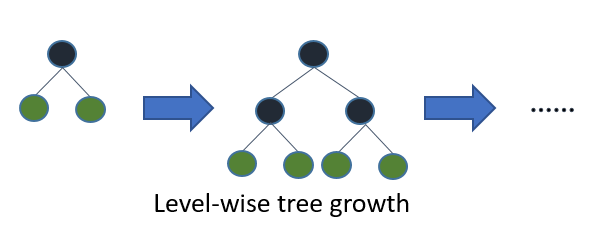
而按叶生长是只针对其中一个叶子节点进行子树生长，并且对该节点进行分叉操作后损失值下降最多。

数学表达如下：

$\begin{array} { l } \left( p _ { m } , f _ { m } , v _ { m } \right) = \arg \min _ { ( p , f , v ) } L \left( T _ { m - 1 } ( X ) . \text { split } ( p , f , v ) , Y \right) \\ T _ { m } ( X ) = T _ { m - 1 } ( X ) . \text { split } \left( p _ { m } , f _ { m } , v _ { m } \right) \end{array}$

在这里插入图片描述

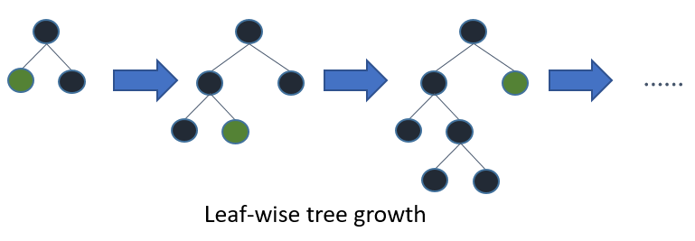
在 LightGBM 中使用的是 leaf-wise 的方法，这样的话在叶子个数一样时，相对于 level-wise 有更高的精度，但是可能会导致生成较深的树，所以 LightGBM 中也提出了限制最大深度来避免过拟合问题。

那么这种使用 leaf-wise tree growth 方法进行决策树的学习的伪代码如下：

$\begin{array} { l } \text {Algorithm : DecisionTree} \\ \text {Input: Training data } ( X , Y ) , \text { number of leaf } C \text { , Loss function } l \\ \triangleright \text { put all data on root } \\ T _ { 1 } ( X ) = X \\ \text {For } m \text { in } ( 2 , C ) \text { : } \\ \qquad \begin{array} { l } \triangleright \text { find best split } \\ \left( p _ { m } , f _ { m } , v _ { m } \right) = \text { FindBestsplit } \left( X , Y , T _ { m - 1 } , l \right) \\ \triangleright \text { perform split } \\ T _ { m } ( X ) = T _ { m - 1 } ( X ) . \text { split } \left( p _ { m } , f _ { m } , v _ { m } \right) \end{array} \end{array}$

其中计算消耗最多的地方是找出最佳的分割点，该分割点查找算法如下：

$\begin{array} { l } \text {Algorithm : FindBestsplit } \\ \text { Input: Training data } ( X , Y ) , \text { Loss function } l \text { , Current Model } T _ { m - 1 } ( X ) \\ \text { For all Leaf } p \text { in } T _ { m - 1 } ( X ) \text { : } \\ \qquad \begin{array}{l} \text { For all } f \text { in X.Features: } \\ \qquad \begin{array}{l} \text { For all } v \text { in f.Thresholds: } \\ \qquad \begin{array}{l} ( \text {left, right} ) = \text {partition} ( p , f , v ) \\ \Delta \operatorname { loss } = L \left( X _ { p } , Y _ { p } \right) - L \left( X _ { \text {left} } , Y _ { \text {left} } \right) - L \left( X _ { \text {right} } , Y _ { \text {right} } \right) \\ \text {if } \Delta \text {loss} > \Delta \operatorname { loss } \left( p _ { m } , f _ { m } , v _ { m } \right) : \\ \left( p _ { m } , f _ { m } , v _ { m } \right) = ( p , f , v ) \end{array} \end{array} \end{array} \end{array}$

那么 LightGBM 便是在此算法上进行的优化。第一个便是直方图算法。

直方图算法（Histogram Algorithm）

回顾 XGBoost 中，是使用预排序算法和加权分位数算法提出的估计分割法，什么意思呢？简单来说就是对数据根据二阶梯度值进行预排序，之后取其分位数 $m\% (N*m=100，n=1,2,\cdots,N)$ ，作为代表或者说采样后代表子集，对该子集穷举选择最优分割点。这样的算法有两个问题：

需要对每个特征按特征值进行排序
由于对特征进行了排序，但梯度并未排序，所以梯度值的获取属于随机内存访问。

这两项都是极其消耗时间和空间的。

具体实现（Implementation）

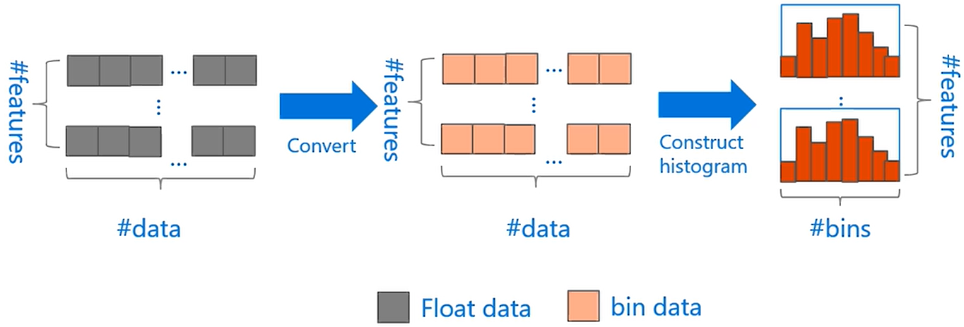
在 LightGBM 中采用了更为高效的方法 —— 直方图算法（Histogram algorithm）。什么意思呢？实际上就是对连续的浮点数据进行分桶操作，或者说离散为 k 个整数值。例如 $\rightarrow 0，[ 0.1,0.3 ) \rightarrow 1$ 。同时 LightGBM 对特征的每个桶进行梯度（一阶和二阶梯度）累加和个数统计。然后根据直方图寻找最优点。下图就是直方图的获取流程：

使用基于直方图的寻找最优分割点时，需要 $\# \text { bin} \times \# \text { feature } )$ 的时间复杂度构建直方图和 $\# \text { data } \times \# \text { feature } )$ 的时间复杂度寻找分割点。直方图算法的伪代码如下：

$\begin{array} { l } \text { Input: } I : \text { training data, } d : \text { max depth } \\ \text { Input: } m : \text { feature dimension } \\ \text { nodeSet } \leftarrow \{ 0 \} \triangleright \text {tree nodes in current level } \\ \text { rowSet } \leftarrow \{ \{ 0,1,2 , \ldots \} \} \triangleright \text {data indices in tree nodes } \\ \text { for } i = 1 \text { to } d \text { do } \\ \qquad\begin{array}{l} \text {for node in nodeSet do } \\ \qquad \begin{array} { l } \text {usedRows } \leftarrow \text {rowSet} [ \text {node} ] \\ \text {for } k = 1 \text { to } m \text { do } \\ \qquad \begin{array}{l} H \leftarrow \text { new Histogram() } \\ \triangleright \text { Build histogram } \\ \text {for } j \text { in usedRows do } \\ \qquad \begin{array}{l} \text {bin } \leftarrow I . f [ \mathrm { k } ] [ \text { j].bin } \\ H [ \text { bin } ] . \mathrm { y } \leftarrow H [ \text { bin } ] . \mathrm { y } + \text { I.y } [ \mathrm { j } ] \\ H [ \text { bin } ] . \mathrm { n } \leftarrow H [ \text { bin } ] . \mathrm { n } + 1 \end{array} \\ \text {Find the best split on histogram } H \\ \cdots \end{array} \end{array} \end{array} \end{array}$

分桶操作（Organization of Bins）

在伪代码中的直方图构建中，分桶操作并没有体现，而是直接获得了该特征值所对应的桶的编号。那这个编号是如何获取的呢，或者说是如何进行分桶操作的呢？实际上这仍然需要一个排序操作，不过只需要在一开始做一步排序获得分桶的分割点即可，之后便可以直接使用桶的分割点对每个特征进行分桶操作了。具体实现在数值类型和类别类型上又不一样。下面介绍一下具体实现。

数值型特征：

对特征值去重后进行排序（从大到小）并统计每个特征值出现的次数 counts。
取 max_bin 和 distinct_value.size 中的较小值作为 bins_num
计算每个桶可以分到的平均样本个数 mean_bin_size，特征取值数 distinct_value.size 比max_bin 数量少，直接取distinct_values的中点作为桶间分割点，即无需分桶。反之则需要分桶，也就是说可能存在几个特征值同分于一个桶中（多特征取值公用一个桶），但是有一点就是当该特征取值的计数值大于平均值 mean_bin_size 时，该特征取值需要单独分桶，所以需要标记出符合该特点的全部特征，之后对不符合的重新计算 mean_bin_size。
然后对于去重后的特征取值进行遍历操作，如果当前的特征需要单独成桶、或者当前桶中个特征计数超过了 mean_bin_size、或者下一个特征是需要独立成桶的，那么当前的特征值将作为当前桶的上界，下一个桶的下界，也就是说需要本步需要结束当前桶的构建，下一步需要建立新的桶了。

看源码涨知识：C++ 中的无穷大数的STL支持std::numeric_limits<double>::infinity()

类别型特征：

首先对特征取值按出现的次数排序（大到小）。
取前 min(max_bin, distinct_values_int.size()) 个特征做特征值到桶之间的映射（这样可能会忽略一些出现次数较少的特征取值），也就是取 max_bin 和 distinct_value.size 中的较小值作为 bins_num。
然后用 bin_2_categorical_（vector类型）记录桶对应的特征取值，以及用categorical_2_bin_(unordered_map类型) 将特征取值对应的桶。

分桶优点（Pros of Bins）

1.内存消耗优化（memory usage optimization），由于无需预排序，并且叶子节点的数据以直方图的形式存储，所以内存消耗可以减小 8 倍以上。

在这里插入图片描述

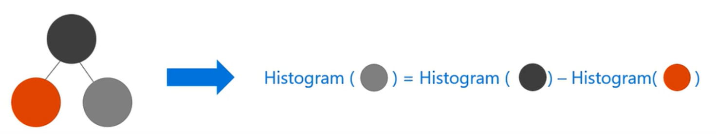
2.利用直方图做差加速特性，在拥有父节点和其中一个子节点的直方图时，可以只消耗 $O(\# \text{bin})$ 的时间复杂度便可以计算得另一节点的直方图。

在这里插入图片描述

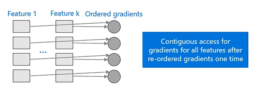
3.提高缓存命中率（Increase cache hit chance），就是优化了内存访问。

回归在 XGBoost 中，需要两种内存随机访问的过程，第一个是梯度值的随机访问，这就不用说了，由于特征的预排序导致的梯度的访问变成了随机内存访问。同时为了提高分割速度，将每个样本点映射到了叶子节点的索引，这样获取该索引时，也是随机内存访问。

在这里插入图片描述

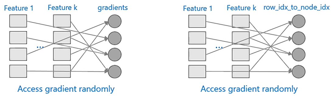
这两处内存的随机访问，导致了效率下降。在 LightGBM 中不需要样本点到叶子节点的索引值，同时各个特征不需要排序，所以是连续内存访问效率更高。

在这里插入图片描述

当然，Histogram算法并不是完美的。由于特征被离散化后，找到的并不是很精确的分割点，所以会对结果产生影响。但在不同的数据集上的结果表明，离散化的分割点对最终的精度影响并不是很大，甚至有时候会更好一点。原因是决策树本来就是弱模型，分割点是不是精确并不是太重要；较粗的分割点也有正则化的效果，可以有效地防止过拟合；即使单棵树的训练误差比精确分割的算法稍大，但在梯度提升（Gradient Boosting）的框架下没有太大的影响。

4.同时由于直方图的特点，在进行数据并行时可大幅降低通信代价（数据并行的实现可见下文）。

算法对比（LightGBM VS XGBoost）

那么基于直方图算法和按叶生长（Leaf-wise tree growth）策略的最佳分割点查找算法实现如下：

$num_of_row) //go through all the data row H[f.bins[i]]. g + = g i ; H[f.bins[i]]. n + = 1 ▹ find best split from histogram For i in (0,len(H)): //go through all the bins S L + = H [ i ] . g ; n L + = H [ i ] . n S R = S P − S L ; n R = n P − n L Δ l o s s = S L 2 n L + S R 2 n R − S P 2 n P if Δ l o s s > Δ l o s s ( p m , f m , v m ) : ( p m , f m , v m ) = ( p , f , H [ i ] . value ) \begin{array} { l } \text { Algorithm: FindBestSplitByHistogram } \\ \text { Input: Training data X, Current Model } T _ { c - 1 } ( X ) \\ \text { First order gradient G, second order gradient H } \\ \text { For all Leaf p in } T _ { c - 1 } ( X ) \text { : } \\ \qquad \begin{array} { l } \text { For all f in X.Features: } \\ \qquad \begin{array} { l } \,\triangleright \text { construct histogram } \\ \text {H = new Histogram() } \\ \text {For i in (0, num\_of\_row) //go through all the data row } \\ \qquad \text { H[f.bins[i]]. } g += g _ { i } ; \text { H[f.bins[i]]. } n + = 1 \\ \,\triangleright \text { find best split from histogram } \\ \text { For i in (0,len(H)): //go through all the bins } \\ \qquad \begin{array} { l } S _ { L } + = H [ i ] . g ; n _ { L } + = H [ i ] . n \\ S _ { R } = S _ { P } - S _ { L } ; n _ { R } = n _ { P } - n _ { L } \\ \Delta l o s s = \frac { S _ { L } ^ { 2 } } { n _ { L } } + \frac { S _ { R } ^ { 2 } } { n _ { R } } - \frac { S _ { P } ^ { 2 } } { n _ { P } } \\ \text {if } \Delta l o s s > \Delta l o s s \left( p _ { m } , f _ { m } , v _ { m } \right) : \\ \qquad \left( p _ { m } , f _ { m } , v _ { m } \right) = ( p , f , H [ i ] . \text { value} ) \end{array} \end{array} \end{array} \end{array}$

与 XGBoost 的对比图如下：

$\begin{array} { c|c | c } \hline & \text { XGBoost } & \text { LightGBM } \\ \hline \text { Tree growth algorithm } & \begin{array} { l } \text { Level-wise good for engineering } \\ \text { optimization , but not efficient } \\ \text { to learn model } \end{array} & \begin{array} { l } \text { Leaf-wise with max depth limitation get } \\ \text { better trees with smaller computation } \\ \text { cost, also can avoid overfitting } \end{array} \\ \hline \text { Split search algorithm } & \text { Pre-sorted algorithm } & \text { Histogram algorithm } \\ \text { memory cost } & \text { 2*\#feature*\#data*4Bytes } & \begin{array} { l } \text { \#feature*\#data*1Bytes (8x smaller) } \end{array} \\ \hline \text { Calculation of split gain } & \text { O(\#data* \#features) } & \text { O(\#bin *\#features) } \\ \hline \text { Cache-line aware optimization } & \text { n/a } & \text { 40\% speed-up on Higgs data } \\ \hline \text { Categorical feature support } & \text { n/a } & \text { 8} \times \text{ speed-up on Expo data } \\ \hline \end{array}$

总体来说 LightGBM 一定程度上优于 XGBoost，实现了不损失精度的前提下提高了训练效率。

基于梯度的单边采样（Gradient-based One-Side Sampling (GOSS)）

除却上述的基本操作外，LightGBM 还针对数据量过大作出以下优化。那对于数据量过大直接解决办法便是减少样本数据量和特征数，所以 LightGBM 据此提出来两个方法：

基于梯度的单边采样（Gradient-based One-Side Sampling (GOSS)）：当对样本进行采样时，为了保持信息增益估计的准确性，应该更好地保留那些具有较大梯度的实例（梯度较大的保留，较小的采样后放大），在相同的目标采样率下，特别是当信息增益的取值范围较大时，这种方法比均匀随机采样能得到更精确的增益估计。
互斥特征捆绑（Exclusive Feature Bundling (EFB)）：通常在实际应用中，虽然特征数量众多，但特征空间相当稀疏，也就是说，在稀疏特征空间中，许多特征（几乎）是相斥的，即它们很少同时取非零值（比如 one-hot 编码）。所以可以安全地捆绑这样的类似的互斥特征。为此，LightGBM 中提出了一个有效的算法，将最优捆绑问题归结为图的着色问题（如果两个特征不是互斥的，则以特征为顶点，每两个特征加一条边），并用一个具有恒定逼近比的贪婪算法求解。

首先针对单边采样进行介绍。其想法是如果一个样本的梯度很小，说明该样本的训练误差很小，或者说该样本已经得到了很好的训练。与 AdaBoost 类似，其会对于分类错误较大的数据样本给予更多的关注。什么意思呢？看一下基于梯度的单边采样（Gradient-based One-Side Sampling (GOSS)）的伪代码：

$\begin{array} { l } \text { Algorithm: Gradient-based One-Side Sampling } \\ \text { Input: } I : \text { training data, } d \text { : iterations } \\ \text { Input: } a : \text { sampling ratio of large gradient data } \\ \text { Input: } b \text { : sampling ratio of small gradient data } \\ \text { Input: } \text {loss:} \text { loss function, } L \text { : weak learner } \\ \text { models } \leftarrow \{ \} , \text { fact } \leftarrow \frac { 1 - a } { b } \\ \text { topN } \leftarrow \mathrm { a } \times \operatorname { len } ( I ) , \operatorname { rand } \mathrm { N } \leftarrow \mathrm { b } \times \operatorname { len } ( I ) \\ \text { for } i = 1 \text { to } d \text { do } \\ \qquad \begin{array}{l} \text { preds } \leftarrow \text { models.predict } ( I ) \\ \, \mathrm { g } \leftarrow los s ( I , \text { preds } ) , \mathrm { w } \leftarrow \{ 1,1 , \ldots \} \\ \text { sorted } \leftarrow \text { GetSortedIndices } ( \mathrm { abs } ( \mathrm { g } ) ) \\ \text { topSet } \leftarrow \text { sorted[1:topN] } \\ \text { randSet } \leftarrow \text { RandomPick(sorted[topN:len(I)], randN) } \\ \text { usedSet } \leftarrow \text { topSet + randSet } \\ \text { w[randSet] } \times = \text { fact } \triangleright \text { Assign weight fact to the small gradient data. } \\ \text { newModel } \leftarrow \mathrm { L } ( I [ \text { usedSet } ] , - \mathrm { g } [ \text { usedSet } ] \text { w[usedSet]) } \\ \text { models.append(newModel) } \end{array} \end{array}$

其中 g 具体的实现是一阶梯度和二阶梯度的乘积。这样通过重新采样的方式可以尽量减小对数据分布的影响。

其具体实现流程如下：

根据梯度的绝对值将样本进行降序排序
选择前a×100%的样本作为 TopSet。
针对剩下的数据(1−a)×100% 的数据进行随机抽取 b×100% 数据组成 RandSet。
由于样本集的减少，在计算增益的时候，选择将 RandSet 所对应的权重放大 (1−a)/b 倍。

那么未使用 GOSS 算法时，在特征 j 上的 d 点进行分割带来的增益如下：

$\frac { 1 } { n _ { O } } \left( \frac { \left( \sum _ { x _ { i } \in O : x _ { i } z d } g _ { i } \right) ^ { 2 } } { n _ { l | l O } ^ { j } ( d ) } + \frac { \left( \sum _ {\left. x _ { i } \in O : x _ { i } \right\rangle d } g _ { i } \right) ^ { 2 } } { n _ { r | O } ^ { j } ( d ) } \right)$

$\text {where } n _ { O } = \sum I \left[ x _ { i } \in O \right] , n _ { l | O } ^ { j } ( d ) = \sum I \left[ x _ { i } \in O : x _ { i j } \leq d \right] \text { and } n _ { r | O } ^ { j } ( d ) = \sum I \left[ x _ { i } \in O : x _ { i j } > d \right]$

那么使用 GOSS 算法后，，在特征 j 上的 d 点进行分割带来的增益变为：

$\frac { 1 } { n _ { O } } \left( \frac { \left( \sum _ { x _ { i } \in A _ { l } } g _ { i } + \frac { 1 - a } { b } \sum _ { x _ { i } \in B _ { l } } g _ { i } \right) ^ { 2 } } { n _ { l } ^ { j } ( d ) } + \frac { \left( \sum _ { x _ { i } \in A _ { r } } g _ { i } + \frac { 1 - a } { b } \sum _ { x _ { i } \in B _ { l } } g _ { r } \right) ^ { 2 } } { n _ { r } ^ { j } ( d ) } \right)$

$\begin{array} { l } \text { where } A _ { l } = \left\{ x _ { i } \in A : x _ { i j } \leq d \right\} , A _ { r } = \left\{ x _ { i } \in A : x _ { i j } > d \right\} , B _ { l } = \left\{ x _ { i } \in B : x _ { i j } \leq d \right\} , B _ { r } = \left\{ x _ { i } \in B : x _ { i j } > d \right\} \\ \text { and the coefficient } \frac { 1 - a } { b } \text { is used to normalize the sum of the gradients over } B \text { back to the size of } A ^ { c } \text { . } \end{array}$

这里 A 代表的是 TopSet，B 代表的是 RandSet。当然在 LightGBM 中也证明了误差收敛性和 GOSS 的泛化性能。

GOSS的估计误差 $\mathcal { E } ( d ) = \left| \tilde { V } _ { j } ( d ) - V _ { j } ( d ) \right|$ 如下：

$\mathcal { E } ( d ) \leq C _ { a , b } ^ { 2 } \ln 1 / \delta \cdot \max \left\{ \frac { 1 } { n _ { l } ^ { j } ( d ) } , \frac { 1 } { n _ { r } ^ { j } ( d ) } \right\} + 2 D C _ { a , b } \sqrt { \frac { \ln 1 / \delta } { n } }$

$\begin{array}{l} \text {where } C _ { a , b } = \frac { 1 - a } { \sqrt { b } } \max _ { x _ { i } \in A ^ { c } } \left| g _ { i } \right| , \text { and } D = \max \left( \bar { g } _ { l } ^ { j } ( d ) , \bar { g } _ { r } ^ { j } ( d ) \right) \\ \text{and }\bar { g } _ { l } ^ { j } ( d ) = \frac { \sum _ { x _ { i } \in \left( A \cup A ^ { c } \right) _ { l } } \left| g _ { i } \right| } { n _ { l } ^ { j } ( d ) } , \bar { g } _ { r } ^ { j } ( d ) = \frac { \sum _ { x _ { i } \in \left( A \cup A ^ { c } \right) _ { r } \left| g _ { i } \right| } } { n _ { r } ^ { j } ( d ) } \end{array}$

该定理证明了 GOSS 的误差估计将在最长 $O (n)$ 的时间复杂度下实现逼近与收敛值。并且当已有数据足够多且分布于全局数据保持一致时，该算法可以保证泛化性能。

互斥特征绑定（Exclusive Feature Bundling）

看到前文的互斥特征绑定定义，我是一头雾水，忍不住把 GBM 读成了 BGM 😅。这实际上针对的是一些特定情境下比如使用 one-hot 编码组成的稀疏数据，这中特征是互斥的（也就是说 one-hot 编码中只有一位为 1 ），而互斥特征绑定（EFB）实际上就是将这些特征绑定在一起，组成一个 bundle，从而实现特征的降维（减小特征数）。如果可实现，那么时间复杂度从 $\# \text { data} \times \# \text { feature } )$ 降低为了 $\# \text { data} \times \# \text { bundle} )$ 。实现上分为两个部分：如何找出互斥特征进行绑定（Greedy Bundling）以及绑定后如何融合（Merge Exclusive Features）。

贪心绑定（Greedy Bundling）

在 LightGBM 论文中已经做出证明，将特征划分为最小数量的互斥 bundle 是 NP 问题。所以这里使用了贪心算法。此算法中使用无向图图表示各特征之间的关系，也就是说图中每个节点表示一个特征，特征之间使用边进行联通成为一个网络，边的权重代表了是否互斥。如果互斥那么代表两个特征可以合并，使用边进行连接。但是由于通常有少量的特征，虽然不是 100% 互斥，并且大多数情况下不会同时取非0值。若构建 Bundle 时允许少量的冲突，就能得到更少数的 bundle，进一步提高效率。可以证明，随机的污染一部分特征的话最多影响训练精度 $\mathcal { O } \left( [ ( 1 - \gamma ) n ] ^ { - 2 / 3 } \right)$ ，其中 $\gamma$ 是最大冲突率，与之相对应的是下面伪代码中的最大冲突个数 $K$ 。所以这里选择将边赋予权重表示节点间的冲突程度，同时类似于前向搜索算法，只是从先向后搜索查找最优解。那么该贪心绑定（Greedy Bundling）的伪代码实现如下：

$\begin{array} { l }\text { Algorithm: Greedy Bundling } \\ \text { Input: } F : \text { features, } K : \text { max conflict count } \\ \text { Construct graph } G \\ \text { searchOrder } \leftarrow G \text { .sortByDegree } ( ) \\ \text { bundles } \leftarrow \{ \} , \text { bundlesconflict } \leftarrow \{ \} \\ \text { for } i \text { in searchOrder do } \\ \qquad \begin{array}{l} \text { needNew } \leftarrow \text { True } \\ \text { for } j = 1 \text { to len(bundles) } \mathbf { d } \mathbf { o } \\ \qquad \begin{array}{l} \text { cnt } \leftarrow \text { Conflict Cnt(bundles[j], } F [ \mathrm { i } ] ) \\ \text { if } c n t + \text { bundlesconflict } [ i ] \leq K \text { then } \\ \qquad \text { bundles[j].add } ( F [ \text { i] } ) , \text { needNew } \leftarrow \text { False } \\ \text { break } \end{array} \\ \text { if needNew then } \\ \qquad \text { Add } F [ i ] \text { as a new bundle to bundles } \end{array} \\ \text { Output: bundles } \end{array}$

具体步骤是：

构建有权无向图，节点是特征，边是节点间的冲突程度
将图按度（知识补充：每个节点边的累加值或者说无权图中节点拥有边的个数）排序
对排序后的节点进行遍历，并判断现存的全部 bundle 是否与本节点符合互斥关系（判断时仍然是从前向后遍历 bundle），符合便加入该 bundle ，反之若不符合建立新的 bundle

该算法的时间复杂度为 $O(\#feature^2)$ ，虽然只需要在训练之前做一次处理，但是当特征数很大的时候，仍然效率不高。对此 LightGBM 提出了一种更为高效的排序策略，直接按特征的非0值的个数进行排序，这与按度排序的策略类似，因为非零值越大意味着冲突的可能性越大。

互斥特征融合（Merge Exclusive Features）

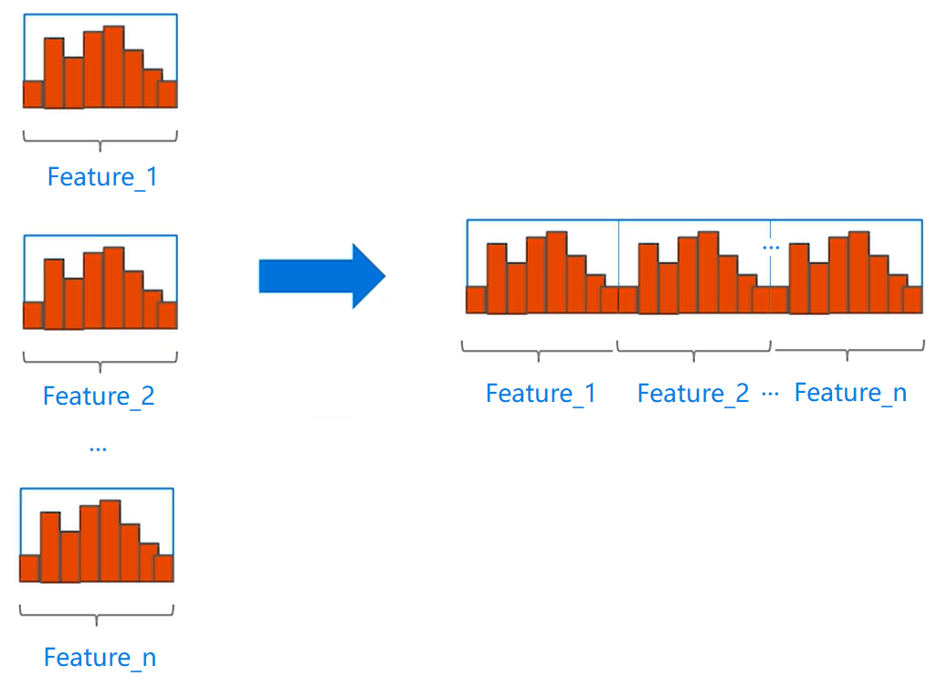
特征融合的关键是原有的不同特征在构建后的 feature bundles 中仍能够识别。由于基于 histogram 的方法存储的是离散的而不是连续的数值,因此可以通过添加偏移的方法将不同特征的 bins 设定在不同的区间。LightGBM 中举出了这样的例子：

Originally, feature A takes value from [0,10) and feature B takes value [0,20) . We then add an offset of 10 to the values of feature B so that the refined feature takes values from [10,30) . After that, it is safe to merge features A and B, and use a feature bundle with range [0,30] to replace the original features A and B.

根据例子可以很容易理解互斥特征融合的技巧，伪代码如下：

$\begin{array} { l }\text { Algorithm: Merge Exclusive Features} \\ \text { Input: } n u m \text { Data: number of data } \\ \text { Input: } F : \text { One bundle of exclusive features } \\ \text { binRanges } \leftarrow \{ 0 \} , \text { totalBin } \leftarrow 0 \\ \text { for } f \text { in } F \text { do } \\ \qquad \text { totalBin } + = \text { f.numBin } \\ \qquad \text { binRanges.append(totalBin) } \\ \text { newBin } \leftarrow \text { new Bin(numData) } \\ \text { for } i = 1 \text { to numData } \mathbf { d } \mathbf { o } \\ \qquad \text { newBin[i] } \leftarrow 0 \\ \qquad \text { for } j = 1 \text { to len} ( F ) \text { do } \\ \qquad \qquad \text { if } F [ j ] . \text { bin } [ i ] \neq 0 \text { then } \\\qquad \qquad \qquad \text { newBin[i] } \leftarrow F [ \text { j].bin[i] + binRanges[j] } \\ \text { Output: newBin, binRanges} \end{array}$

具体步骤是：在该 bundle 中，将当前特征前已遍历的全部特征拥有的桶的总个数作为偏移量，将全部的特征的桶进行直方图合并，示意图如下：

在这里插入图片描述

EFB算法可以将大量的互斥特征捆绑到较少的密集特征上，有效地避免了对零特征值的不必要计算。同时实际上，也可以通过为每个特征使用一个表来记录具有非零值的数据，忽略零特征值，进而达到优化基本的基于直方图的算法的目的。通过扫描此表中的数据，特征的直方图构建成本将从 $O(\#data)$ 更改为 $O(\#non\_zero\_data)$ 。然而，这种方法需要额外的内存和计算开销来维护整个树生长过程中的每个特征表。LightGBM 将这个优化方法集成为了一个基本函数来实现。注意，这个优化与 EFB 并不冲突，因为当 bundle 稀疏时仍然可以使用它。

并行学习的优化（Optimization in Parallel Learning）

并行计算在 LightGBM 的官方文档中和微软亚洲研究院发布的视频如何玩转LightGBM 都做了介绍，这里我便简单的翻译和记录一下，不再写具体的证明。

特征并行（Feature Parallel）

在这里插入图片描述

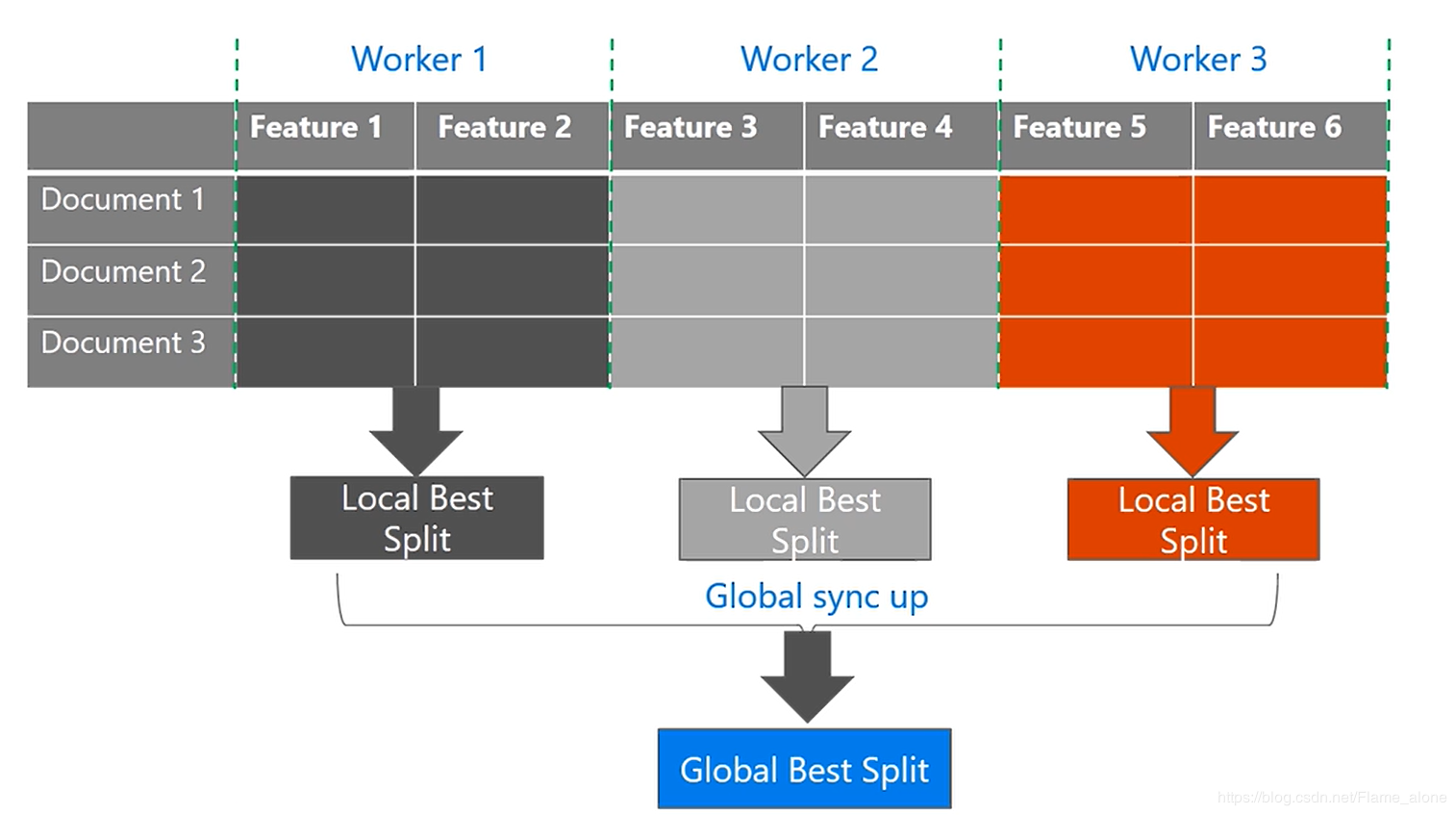
特征并行主要针对的是数据量较小、特征较多的情景。其是通过垂直的切分数据，使得全部机器上都有所有的数据样本点，但是不同机器上所存储的特征不一样，这样每个机器都计算出该机器上可以获得的最优的局部分割点，然后通过全部的局部最优分割点获得全局最优分割点。

数据并行（Data Parallel）

在这里插入图片描述

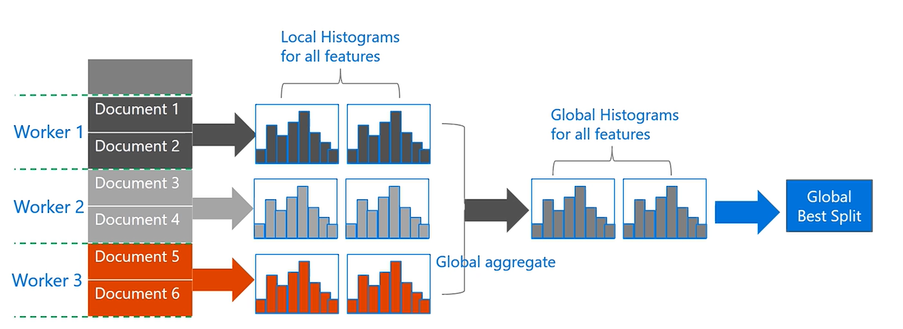
数据并行主要针对的是数据量比较大、特征较少的情景。其是通过水平的切分数据，全部机器上拥有部分的数据样本点，但是包含全部的特征，这样每个机器可以构造出全部特征的局部（本地）直方图，然后通过全部的局部直方图获取全局的全部特征的直方图，在后在全局直方图上查找最优分割点。

投票并行（Voting Parallel）

在这里插入图片描述

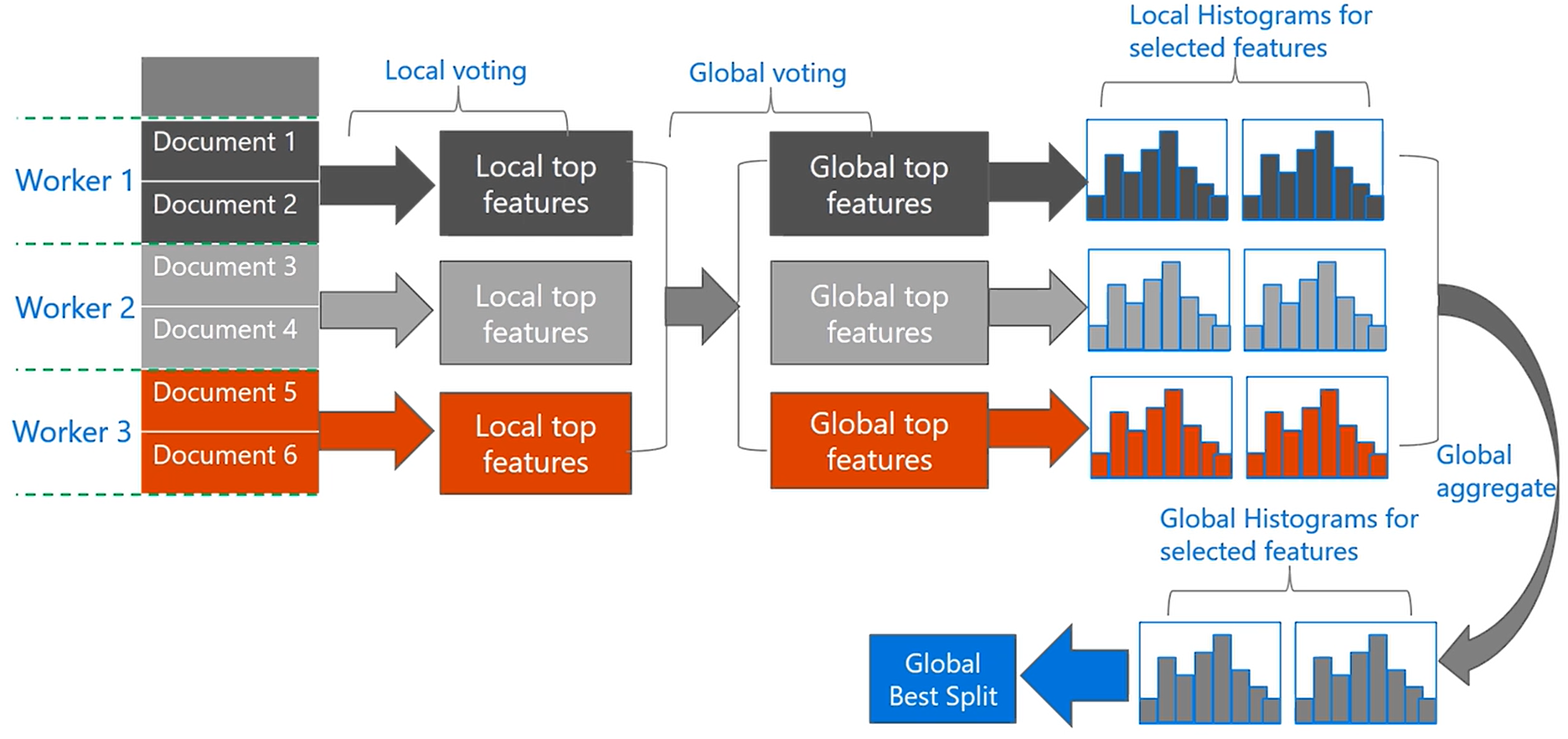
投票并行主要针对数据量较大、特征较多的情景。主要是针对使用数据并行时，特征直方图合并导致的通讯消耗。这里通过二阶段投票的方式只合并部分直方图来弥补这一缺陷。首先是通过本地的数据找出（局部投票获得） Top k 的最优特征（用于分割），然后将这些特征整合在一起，并对这些特征通过全局投票获取到可能是全局最优分割点的 Top 2*K 特征，之后只针对这些特征进行直方图的合并。

LightGBM采用一种称为 PV-Tree 的算法进行投票并行(Voting Parallel)其实这本质上也是一种数据并行。PV-Tree 和普通的决策树差不多,只是在寻找最优切分点上有所不同。

具体的算法伪代码如下：

$\begin{array} { l } \text { Algorithm : PV-Tree FindBestSplit}\\ \text { Input: Dataset } D \\ \text { localHistograms = ConstructHistograms(D) } \\ \,\, \triangleright \text { Local Voting } \\ \text { splits = [] } \\ \text { for all H in localHistograms do } \\ \qquad \text { splits.Push(H.FindBestSplit()) } \\ \text { end for } \\ \text { localTop = splits.TopKByGain(K) } \\ \,\, \triangleright \text { Gather all candidates } \\ \text { allCandidates = AllGather(localTop) } \\ \,\, \triangleright \text { Global Voting } \\ \text { globalTop = allCandidates.TopKByMajority(2*K) } \\ \,\, \triangleright \text { Merge global histograms } \\ \text { globalHistograms = Gather(globalTop, localHistograms) } \\ \text { bestSplit = globalHistograms.FindBestSplit() } \\ \text { return bestSplit } \end{array}$

代码中的 FindBestSplit 函数也就是单机运行函数实现如下：

$\begin{array} { l } \text { Algorithm : FindBestSplit}\\ \text { Input: DataSet } \\ \text { for all } \mathrm { X } \text { in D.Attribute } \mathrm { d } \mathbf { o } \\ \qquad \begin{array} { l } \,\, \triangleright \text { Construct Histogram } \\ \text { H = new Histogram() } \\ \text { for all } \mathrm { x } \text { in } \mathrm { X } \text { do } \\ \qquad \text { H.binAt(x.bin).Put(x.label) } \\ \text { end for } \\ \,\, \triangleright \text { Find Best Split } \\ \text { leftSum = new HistogramSum() } \\ \text { for all bin in H do } \\ \qquad \begin{array} { l } \text { leftSum = leftSum + H.binAt(bin) } \\ \text { rightSum = H.AllSum - leftSum } \\ \text { split.gain = CalSplitGain(leftSum, rightSum) } \\ \text { bestSplit = ChoiceBetterOne(split,bestSplit) } \end{array} \\ \text { end for } \end{array} \\ \text { end for } \\ \text { return bestSplit } \end{array}$

使用经验（Hands-on Experience）

更快的学习速度（Faster Learining Speed）

使用 bagging 操作，对数据进行采用（子集）
对特征进行子集采用
可以直接使用类别特征无需离散化
将数据存为二进制数据文件，这样在多次训练时可以做到更快
使用并行学习

更好的精度（Better Accuracy）

较小的学习率和较多的迭代次数
较多叶子的个数
交叉验证
更多的训练数据
Try DART-use drop out during the training

处理过拟合（Deal with Overfitting）

small maxbin_feature——分桶略微粗一些
small num_leaves——不要在单棵树上分的太细
Control min_data_in_leaf and min_sum_hessian_in_leaf——确保叶子节点还有足够多的数据
Sub - sample——在构建每棵树的时候,在data上做一些 sample
Sub - feature——在构建每棵树的时候,在feature上做一些 sample
bigger training data——更多的训练数据
lambda, lambda_l2 and min_gaint_ split to regularization——正则
max_ depth to avoid growing deep tree——控制树深度

参考论文：LightGBM: A Highly Efficient Gradient Boosting Decision Tree

参考视频：如何玩转LightGBM，集成学习：XGBoost, lightGBM。

FlameAlpha

关注

53
点赞
踩
180

收藏

觉得还不错? 一键收藏
打赏
8
评论
梯度提升机（Gradient Boosting Machine）之 LightGBM

随着大数据时代的到来，GBDT正面临着新的挑战，特别是在精度和效率之间的权衡方面。传统的GBDT实现需要对每个特征扫描所有数据实例，以估计所有可能的分割点的信息增益。因此，它们的计算复杂度将与特征数和实例数成正比。这使得这些实现在处理大数据时非常耗时。直接的想法是减少样本数据量和特征数。LightGBM 针对这两种操作提出来两个方法：基于梯度的单边采样（Gradient-based One-Side Sampling (GOSS)）：当对样本进行采样时，为了保持信息增益估计的准确性，应该更好地保留那些
复制链接

扫一扫