tensorflow保存和恢复模型的两种方法介绍

一、前言

本文将会介绍tensorflow保存和恢复模型的两种方法，一种是传统的Saver类save保存和restore恢复方法，还有一种是比较新颖的SavedModelBuilder类的builder保存和loader文件里的load恢复方法。通过了解这两种方法，我们可以解决如何保存和恢复一个已经训练好的神经网络模型用于推理预测的现实需求，也可以辅助查看分析一个长时间训练的模型性能，最重要的是我们可以预防因长时间训练中途出现断电、宕机、出错退出等问题导致的训练功亏一篑问题！可见，掌握tensorflow保存和恢复模型的方法，对我们工程应用有多么大的帮助，同时，这也是我们必须要掌握的基础技能，下面我将分别介绍它们！

二、模型保存恢复之save/restore方法

save和restore方法主要在Saver类里实现，源代码位于tensorflow/python/training/saver.py

 

2-1）不管是save还是restore，我们首先都是要新建一个Saver，使用方法如下：

saver = tf.train.Saver(...)

注意一点：位于 tf.train.Saver()之后的变量将不会被存储!

Saver的构造函数如下：

__init__(
    var_list=None,
    reshape=False,
    sharded=False,
    max_to_keep=5,
    keep_checkpoint_every_n_hours=10000.0,
    name=None,
    restore_sequentially=False,
    saver_def=None,
    builder=None,
    defer_build=False,
    allow_empty=False,
    write_version=tf.train.SaverDef.V2,
    pad_step_number=False,
    save_relative_paths=False,
    filename=None
)

对我们来说比较关注的有以下几个配置参数：

保存模型时：

var_list：特殊需要保存和恢复的变量和可保存对象列表或字典，默认为空，将会保存所有的可保存对象；

max_to_keep：保存多少个最新的checkpoint文件，默认为5，即保存最近五个checkpoint文件；

keep_checkpoint_every_n_hours：多久保存checkpoint文件，默认为10000小时，相当于禁用了这个功能；

save_relative_paths：为True时，checkpoint文件将不会记录完整的模型路径，而只会仅仅记录模型名字，这方便于将保存下来的模型复制到其他目录并使用的情况；

 

恢复模型时：

reshape：为True时，允许从已保存checkpoint文件里恢复并重新设定形状不一样的张量，默认为false；

sharded：碎片化checkpoint文件到每一个设备，默认false；

restore_sequentially：为True时，会在每个设备中顺序地恢复不同的变量，同时可以在恢复比较大的模型时节省内存；

 

2-2）使用Saver类的save接口保存模型

saver.save(...)

save接口如下：

save(
    sess,
    save_path,
    global_step=None,
    latest_filename=None,
    meta_graph_suffix='meta',
    write_meta_graph=True,
    write_state=True
)

该方法运行为保存变量的构造函数所添加的ops，它需要一个已经建好图的会话，同时要求所有变量均已经被初始化，该函数返回保存模型的绝对路径，可用于restore时使用。

其参数说明如下：

sess：一个建好图的会话，用以运行保存操作；

save_path：包含模型名字的绝对路径，最终会自动在模型名字添加相应后缀

global_step：该参数会自动添加到save_path名字用以区别不同步骤保存的模型；

latest_filename：生成检查点文件的名字，默认是“checkpoint”；

meta_graph_suffix：MetaGraphDef元图后缀，默认为“meta”；

write_meta_graph：指明是否要保存元图数据，默认为True；

write_state：指明是否要写CheckpointStateProto，默认为True；

 

2-3）获取最近保存的所有模型

last_ckpt = saver.last_checkpoints

或者使用如下方法：

# get_checkpoint_state(checkpoint_dir, latest_filename=None)
ckpt = tf.train.get_checkpoint_state("/home/xsr-ai/study/mnist/mnist-model")

这将会得到一个包含有最近保存模型的列表，但是不包括checkpoint检查点文件，如下；

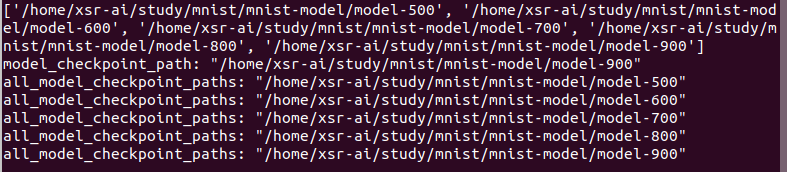
我们要恢复哪一个模型，可以使用如下任一种类似方法：

saver.restore(last_ckpt[-1])
saver.restore(last_ckpt[0])
saver.restore(ckpt.model_checkpoint_path)
saver.restore(ckpt.all_model_checkpoint_paths[-1])

 

2-4）使用restore恢复已保存模型

saver.restore(sess, save_path)

该函数恢复一个已保存的模型，它需要一个已建好图结构的会话，恢复模型得到的变量无需初始化，在恢复过程中已有对保存变量做了初始化操作。

sess：用以恢复参数模型的会话；

save_path：已保存模型的路径，通常包含模型名字；

 

2-5）图存储和加载write_graph/import_graph_def方法

有时候我们建立好一个会话图后，需要保存，以供将来使用，那么以下方法是很有效的！

 

图存储方法：

def write_graph(graph_or_graph_def, logdir, name, as_text=True):

该函数存储一个tensorflow图原型到文件里，其参数含义如下：

graph_or_graph_def：tensorflow Graph或GraphDef；

logdir：保存图或图原型的目录；

as_text：默认为True，即以ASCII方式写到文件里

return：返回图或图原型保存的路径

使用例子如下：

v = tf.Variable(0, name='my_variable')
sess = tf.Session()
# tf.train.write_graph(sess.graph, '/tmp/my-model', 'train.pbtxt') --> that is ok
tf.train.write_graph(sess.graph_def, '/tmp/my-model', 'train.pbtxt')

 

图加载方法：

def import_graph_def(graph_def, input_map=None, return_elements=None, name=None, op_dict=None, producer_op_list=None):

该函数可加载已存储的"graph_def"到当前默认图里，并从系列化的tensorflow [`GraphDef`]协议缓冲里提取所有的tf.Tensor和tf.Operation到当前图里，其参数如下：

graph_def：一个包含图操作OP且要导入GraphDef的默认图；

input_map：字典关键字映射，用以从已保存图里恢复出对应的张量值；

return_elements：从已保存模型恢复的Ops或Tensor对象；

return：从已保存模型恢复后的Ops和Tensorflow列表，其名字位于return_elements；

使用例子如下：

with tf.Session() as _sess:
  with gfile.FastGFile("/tmp/tfmodel/train.pbtxt",'rb') as f:
    graph_def = tf.GraphDef()
    graph_def.ParseFromString(f.read())
    _sess.graph.as_default()
    tf.import_graph_def(graph_def, name='tfgraph')

 

2-6）MetaGraph导出和导入export_meta_graph/ import_meta_graph方法

先了解一下什么是MetaGraph：

一个MetaGraph既包含了tensorflow GraphDef，也包含了在跨越进程边界时在图形中运行计算所需的相关元数据，它也可以用来长期存储tensorflow图结构。MetaGraph包含继续训练、执行评估或在先前训练的图形上运行推理所需的信息。

MetaGraph包含的信息被表示为一个MetaGraphDef协议缓冲，它包含如下几方面：

MetaInfoDef：元信息，比如版本信息和用户信息；

GraphDef：用于描述一个图结构；

SaverDef：用于Saver；

CollectionDef ：映射进一步描述模型的其他组件，比如变量或tensorflow队列；

 

MetaGraph导出方法：

def export_meta_graph(filename=None, collection_list=None, as_text=False, export_scope=None, clear_devices=False, clear_extraneous_savers=False):

该函数可以导出tensorflow元图及其所需的数据,其参数如下：

filename：保存路径及其文件名；

collection_list：要收集的字符串键的列表；

as_text：为True时导出的文本格式为ASCII编码；

export_scope：导出的名字空间，用以删除；

clear_devices：导出时将与设备相关的信息去掉，即导出文件不与特定设备环境关联；

clear_extraneous_savers：从图中删除与此导出操作无关的任何saver相关信息(保存/恢复操作和SaverDefs)。

return：MetaGraphDef proto；

官方提供的使用例程：

# Build the model
...
with tf.Session() as sess:
  # Use the model
  ...
# Export the default running graph and only a subset of the collections.
meta_graph_def = tf.train.export_meta_graph(
    filename='/tmp/my-model.meta',
    collection_list=["input_tensor", "output_tensor"])

 

MetaGraph导入方法：

def import_meta_graph(meta_graph_or_file, clear_devices=False, import_scope=None, **kwargs):

该函数以“MetaGraphDef”协议缓冲区作为输入，如果其参数是一个包含“MetaGraphDef”协议缓冲区的文件，它将以文件内容构造一个协议缓冲区，然后将“graph_def”字段中的所有节点添加到当前图形，并重新创建所有由collection_list收集的列表内容，最后返回由“saver_def”字段构造的saver以供使用，其参数如下：

meta_graph_or_file：`MetaGraphDef`协议缓冲区或者包含MetaGraphDef且带有路径的文件名；

clear_devices：导入时将与设备相关的信息去掉，即不与导出时的图设备环境关联，可兼容当前设备环境；

import_scope：导入名字空间，用以删除；

**kwargs：可选的参数；

return：在“MetaGraphDef”中由“saver_def”构造的存储模型，如果MetaGraphDef没有保存的变量则会直接返回None；

官方提供的使用例程：

...
# Create a saver.
saver = tf.train.Saver(...variables...)
# Remember the training_op we want to run by adding it to a collection.
tf.add_to_collection('train_op', train_op)
sess = tf.Session()
for step in xrange(1000000):
    sess.run(train_op)
    if step % 1000 == 0:
        # Saves checkpoint, which by default also exports a meta_graph
        # named 'my-model-global_step.meta'.
        saver.save(sess, 'my-model', global_step=step)


with tf.Session() as sess:
  new_saver = tf.train.import_meta_graph('my-save-dir/my-model-10000.meta')
  new_saver.restore(sess, 'my-save-dir/my-model-10000')
  # tf.get_collection() returns a list. In this example we only want the
  # first one.
  train_op = tf.get_collection('train_op')[0]
  for step in xrange(1000000):
    sess.run(train_op)

三、举例说明save/restore方法

下面我们将基于mnist写一个例子来说明如何使用save/restore方法保存和恢复模型，这是一个基于softmax的mnist例程，为了执行这个程序，我们需要事先下载mnist数据，可到网站

MNIST handwritten digit database, Yann LeCun, Corinna Cortes and Chris Burges下载

执行命令时需要指定命令行参数“--data_dir”到你存放mnist数据的目录，例如：

python mnist_softmax.py --data_dir /home/xsr-ai/study/mnist/

"""A very simple MNIST classifier.

See extensive documentation at
https://www.tensorflow.org/get_started/mnist/beginners
"""
from __future__ import absolute_import
from __future__ import division
from __future__ import print_function

import argparse
import sys

from tensorflow.examples.tutorials.mnist import input_data

import tensorflow as tf

FLAGS = None


def main(_):
  # Import data
  mnist = input_data.read_data_sets(FLAGS.data_dir, one_hot=True)

  # Create the model
  x = tf.placeholder(tf.float32, [None, 784])
  W = tf.Variable(tf.zeros([784, 10]))
  b = tf.Variable(tf.zeros([10]))
  y = tf.matmul(x, W) + b

  # Define loss and optimizer
  y_ = tf.placeholder(tf.float32, [None, 10])

  # The raw formulation of cross-entropy,
  #
  #   tf.reduce_mean(-tf.reduce_sum(y_ * tf.log(tf.nn.softmax(y)),
  #                                 reduction_indices=[1]))
  #
  # can be numerically unstable.
  #
  # So here we use tf.nn.softmax_cross_entropy_with_logits on the raw
  # outputs of 'y', and then average across the batch.
  cross_entropy = tf.reduce_mean(
      tf.nn.softmax_cross_entropy_with_logits(labels=y_, logits=y))
  train_step = tf.train.GradientDescentOptimizer(0.5).minimize(cross_entropy)

  sess = tf.InteractiveSession()
  tf.global_variables_initializer().run()
  # Train
  saver = tf.train.Saver()
  for index in range(1000):
    batch_xs, batch_ys = mnist.train.next_batch(100)
    sess.run(train_step, feed_dict={x: batch_xs, y_: batch_ys})
    if index % 100 == 0:
      print("index: %d" % index)
      path = saver.save(sess, "/home/xsr-ai/study/mnist/mnist-model/model.ckpt", global_step=index) # , latest_filename="hello"

  # Test trained model
  correct_prediction = tf.equal(tf.argmax(y, 1), tf.argmax(y_, 1))
  accuracy = tf.reduce_mean(tf.cast(correct_prediction, tf.float32))
  print(sess.run(accuracy, feed_dict={x: mnist.test.images,
                                      y_: mnist.test.labels}))
 
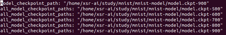
  ckpt = tf.train.get_checkpoint_state("/home/xsr-ai/study/mnist/mnist-model")
  saver.restore(sess, ckpt.all_model_checkpoint_paths[0])
  print(ckpt)
  print(sess.run(accuracy, feed_dict={x: mnist.test.images,
                                      y_: mnist.test.labels}))

if __name__ == '__main__':
  parser = argparse.ArgumentParser()
  parser.add_argument('--data_dir', type=str, default='/tmp/tensorflow/mnist/input_data',
                      help='Directory for storing input data')
  FLAGS, unparsed = parser.parse_known_args()
  tf.app.run(main=main, argv=[sys.argv[0]] + unparsed)

执行如上程序会得到如下终端打印信息：

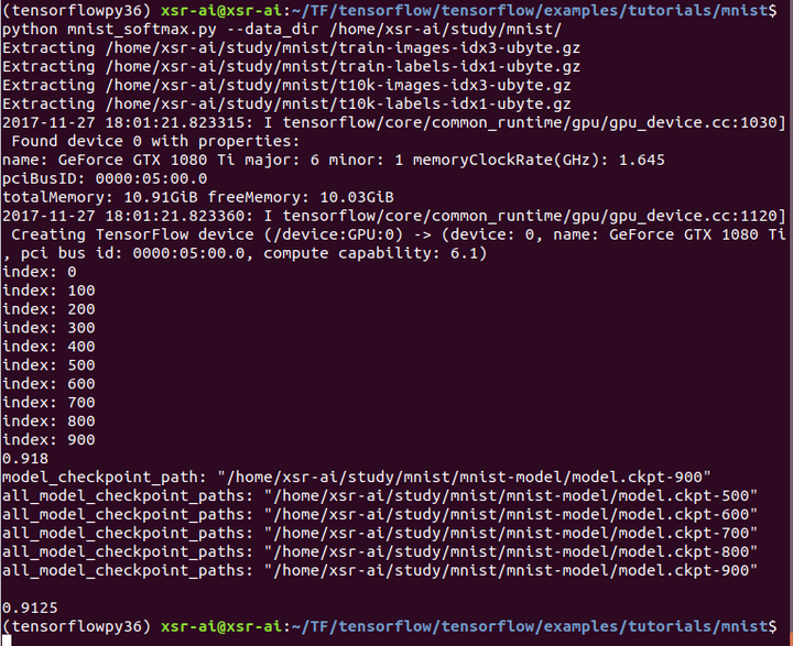
我们看到准确率并不是很高，那是我们没有使用包含空间信息的卷积神经网络结构来训练，同时在模型保存的目录下面出现几个保存的模型：

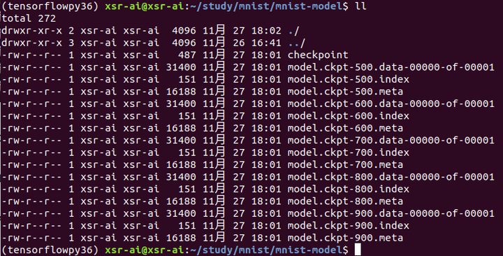
包含一个checkpoint文件，它记录了max_to_keep个最新的保存模型信息，如下：

同时，按照默认max_to_keep等于5则包含五个模型信息，其中有 5 个 model.ckpt-{global_step}.data-00000-of-00001 文件,是训练过程中保存的模型,5 个 model.ckpt-{global_step}.meta 文件,是训练过程中保存的元数据(TensorFlow 默认只保存最近 5 个模型和元数据,删除前面没用的模型和元数据),5 个 model.ckpt-{global_step}.index 文件，{global_step}代表迭代次数。

实际上，我有在程序后面使用saver.restore方法恢复了保存的模型，然后进行了预测：

ckpt = tf.train.get_checkpoint_state("/home/xsr-ai/study/mnist/mnist-model")
  saver.restore(sess, ckpt.all_model_checkpoint_paths[0])
  print(ckpt)
  print(sess.run(accuracy, feed_dict={x: mnist.test.images,
                                      y_: mnist.test.labels}))

因为使用的模型是五个中比较早并非最近的一个，所以预测准确率只有0.9125，这比最后一次预测的准确率0.918要差一点点的。

四、模型保存恢复之builder/loader方法

builder/loader方法也是可以保存和恢复tensorflow模型的，只是他们源代码是在不同文件里，builder其源代码在tensorflow/python/saved_model/builder_impl.py，而loader的源代码则位于tensorflow/python/saved_model/loader_impl.py。相较于save和restore方法会生成比较多的模型文件，builder和loader方法则会更简单一些，同时也是saver提供的更高级别的系列化，它也更适合于商业化，按照创作者的说法“它显然是未来！”

 

使用builder方法保存模型：

我们主要使用SavedModelBuilder类来新建一个builder，SavedModelBuilder的参数很简单，就一个export_dir参数即要保存模型的路径，但要确保所保存的目录是未有建立的，否则会导致出错！

获取builder方法如下：

builder = tf.saved_model.builder.SavedModelBuilder("/home/xsr-ai/study/mnist/saved-model")

在训练完后，我们调用如下命令保存模型：

builder.add_meta_graph_and_variables(sess, [tf.saved_model.tag_constants.TRAINING], signature_def_map=None, assets_collection=None)
builder.save()

add_meta_graph_and_variables的介绍如下：

def add_meta_graph_and_variables(sess,tags,signature_def_map=None,assets_collection=None,legacy_init_op=None,clear_devices=False,main_op=None):

该函数可以将当前元图添加到SavedModel并保存变量，其参数如下：

sess：用于执行添加元图和变量功能的会话；

tags：用于保存元图的标签；

signature_def_map：用于保存元图的签名；

assets_collection：使用SavedModel保存的资源集合；

legacy_init_op：在恢复模型操作后，对Op和Ops组的遗留支持；

clear_devices：如果默认图形上的设备信息应该被清除，则应该设置为true；

main_op：在加载图时执行Op或Ops组的操作。请注意，当main_op被指定时，它将在加载恢复op后运行；

return：无返回

 

save()的介绍：

def save(as_text=False):

该函数将“SavedModel”协议缓冲区的数据写入到硬盘里，其参数只有一个as_text，主要用于指明是否按照ASCII编码格式写入到文件里，其返回的是保存模型的路径。

 

使用loader方法恢复模型：

我们主要使用load(...)来恢复模型：

def load(sess, tags, export_dir, **saver_kwargs):

该函数可以从标签指定的SavedModel加载模型，其参数如下：

sess：恢复模型的会话；

tags：用于恢复元图的标签，需与保存时的一致，用于区别不同的模型；

export_dir：存储SavedModel协议缓冲区和要加载的变量的目录；

**saver_kwargs：可选的关键字参数传递给saver；

return：在提供的会话中加载的“MetaGraphDef”协议缓冲区，这可以用于进一步提取signature-defs, collection-defs等；

 

load通常使用方法如下：

with tf.Session() as sess:  
    tf.saved_model.loader.load(sess, [tf.saved_model.tag_constants.TRAINING], "/home/xsr-ai/study/mnist/saved-model")

一定要注意标签和模型路径都要与保存模型时一致，然后使用相应的变量时，需要保存时的名字空间！

五、举例说明builder/loader方法

与save/restore方法一样，我们也用mnist来举例说明如何使用builder/loader方法来保存恢复模型,但这次我们用卷积神经网络的方法，顺便看看准确率是不是有很大的提高！

"""A simple MNIST classifier which displays summaries in TensorBoard.

This is an unimpressive MNIST model, but it is a good example of using
tf.name_scope to make a graph legible in the TensorBoard graph explorer, and of
naming summary tags so that they are grouped meaningfully in TensorBoard.

It demonstrates the functionality of every TensorBoard dashboard.
"""
from __future__ import absolute_import
from __future__ import division
from __future__ import print_function

import argparse
import os
import sys

import tensorflow as tf

from tensorflow.examples.tutorials.mnist import input_data

FLAGS = None


def train():
  # Import data
  mnist = input_data.read_data_sets(FLAGS.data_dir,
                                    one_hot=True,
                                    fake_data=FLAGS.fake_data)

  sess = tf.InteractiveSession()
  # Create a multilayer model.

  # Input placeholders
  with tf.name_scope('input'):
    x = tf.placeholder(tf.float32, [None, 784], name='x-input')
    y_ = tf.placeholder(tf.float32, [None, 10], name='y-input')

  with tf.name_scope('input_reshape'):
    image_shaped_input = tf.reshape(x, [-1, 28, 28, 1])
    tf.summary.image('input', image_shaped_input, 10)

  # We can't initialize these variables to 0 - the network will get stuck.
  def weight_variable(shape):
    """Create a weight variable with appropriate initialization."""
    initial = tf.truncated_normal(shape, stddev=0.1)
    return tf.Variable(initial)

  def bias_variable(shape):
    """Create a bias variable with appropriate initialization."""
    initial = tf.constant(0.1, shape=shape)
    return tf.Variable(initial)

  def variable_summaries(var):
    """Attach a lot of summaries to a Tensor (for TensorBoard visualization)."""
    with tf.name_scope('summaries'):
      mean = tf.reduce_mean(var)
      tf.summary.scalar('mean', mean)
      with tf.name_scope('stddev'):
        stddev = tf.sqrt(tf.reduce_mean(tf.square(var - mean)))
      tf.summary.scalar('stddev', stddev)
      tf.summary.scalar('max', tf.reduce_max(var))
      tf.summary.scalar('min', tf.reduce_min(var))
      tf.summary.histogram('histogram', var)

  def nn_layer(input_tensor, input_dim, output_dim, layer_name, act=tf.nn.relu):
    """Reusable code for making a simple neural net layer.

    It does a matrix multiply, bias add, and then uses ReLU to nonlinearize.
    It also sets up name scoping so that the resultant graph is easy to read,
    and adds a number of summary ops.
    """
    # Adding a name scope ensures logical grouping of the layers in the graph.
    with tf.name_scope(layer_name):
      # This Variable will hold the state of the weights for the layer
      with tf.name_scope('weights'):
        weights = weight_variable([input_dim, output_dim])
        variable_summaries(weights)
      with tf.name_scope('biases'):
        biases = bias_variable([output_dim])
        variable_summaries(biases)
      with tf.name_scope('Wx_plus_b'):
        preactivate = tf.matmul(input_tensor, weights) + biases
        tf.summary.histogram('pre_activations', preactivate)
      activations = act(preactivate, name='activation')
      tf.summary.histogram('activations', activations)
      return activations

  hidden1 = nn_layer(x, 784, 500, 'layer1')

  with tf.name_scope('dropout'):
    keep_prob = tf.placeholder(tf.float32)
    tf.summary.scalar('dropout_keep_probability', keep_prob)
    dropped = tf.nn.dropout(hidden1, keep_prob)

  # Do not apply softmax activation yet, see below.
  y = nn_layer(dropped, 500, 10, 'layer2', act=tf.identity)

  with tf.name_scope('cross_entropy'):
    # The raw formulation of cross-entropy,
    #
    # tf.reduce_mean(-tf.reduce_sum(y_ * tf.log(tf.softmax(y)),
    #                               reduction_indices=[1]))
    #
    # can be numerically unstable.
    #
    # So here we use tf.nn.softmax_cross_entropy_with_logits on the
    # raw outputs of the nn_layer above, and then average across
    # the batch.
    diff = tf.nn.softmax_cross_entropy_with_logits(labels=y_, logits=y)
    with tf.name_scope('total'):
      cross_entropy = tf.reduce_mean(diff)
  tf.summary.scalar('cross_entropy', cross_entropy)

  with tf.name_scope('train'):
    train_step = tf.train.AdamOptimizer(FLAGS.learning_rate).minimize(
        cross_entropy)

  with tf.name_scope('accuracy'):
    with tf.name_scope('correct_prediction'):
      correct_prediction = tf.equal(tf.argmax(y, 1), tf.argmax(y_, 1))
    with tf.name_scope('accuracy'):
      accuracy = tf.reduce_mean(tf.cast(correct_prediction, tf.float32))
  tf.summary.scalar('accuracy', accuracy)

  # Merge all the summaries and write them out to
  # /tmp/tensorflow/mnist/logs/mnist_with_summaries (by default)
  merged = tf.summary.merge_all()
  train_writer = tf.summary.FileWriter(FLAGS.log_dir + '/train', sess.graph)
  test_writer = tf.summary.FileWriter(FLAGS.log_dir + '/test')
  tf.global_variables_initializer().run()

  # Train the model, and also write summaries.
  # Every 10th step, measure test-set accuracy, and write test summaries
  # All other steps, run train_step on training data, & add training summaries

  def feed_dict(train):
    """Make a TensorFlow feed_dict: maps data onto Tensor placeholders."""
    if train or FLAGS.fake_data:
      xs, ys = mnist.train.next_batch(100, fake_data=FLAGS.fake_data)
      k = FLAGS.dropout
    else:
      xs, ys = mnist.test.images, mnist.test.labels
      k = 1.0
    return {x: xs, y_: ys, keep_prob: k}

  for i in range(FLAGS.max_steps):
    if i % 100 == 0:  # Record summaries and test-set accuracy
      summary, acc = sess.run([merged, accuracy], feed_dict=feed_dict(False))
      test_writer.add_summary(summary, i)
      print('Accuracy at step %s: %s' % (i, acc))
    else:  # Record train set summaries, and train
      if i % 100 == 99:  # Record execution stats
        run_options = tf.RunOptions(trace_level=tf.RunOptions.FULL_TRACE)
        run_metadata = tf.RunMetadata()
        summary, _ = sess.run([merged, train_step],
                              feed_dict=feed_dict(True),
                              options=run_options,
                              run_metadata=run_metadata)
        train_writer.add_run_metadata(run_metadata, 'step%03d' % i)
        train_writer.add_summary(summary, i)
        print('Adding run metadata for', i)
      else:  # Record a summary
        summary, _ = sess.run([merged, train_step], feed_dict=feed_dict(True))
        train_writer.add_summary(summary, i)

  builder = tf.saved_model.builder.SavedModelBuilder("/home/xsr-ai/study/mnist/saved-model")
  builder.add_meta_graph_and_variables(sess, [tf.saved_model.tag_constants.TRAINING])
  builder.save()  

  train_writer.close()
  test_writer.close()


def main(_):
  if tf.gfile.Exists(FLAGS.log_dir):
    tf.gfile.DeleteRecursively(FLAGS.log_dir)
  tf.gfile.MakeDirs(FLAGS.log_dir)
  train()


if __name__ == '__main__':
  parser = argparse.ArgumentParser()
  parser.add_argument('--fake_data', nargs='?', const=True, type=bool,
                      default=False,
                      help='If true, uses fake data for unit testing.')
  parser.add_argument('--max_steps', type=int, default=1000,
                      help='Number of steps to run trainer.')
  parser.add_argument('--learning_rate', type=float, default=0.001,
                      help='Initial learning rate')
  parser.add_argument('--dropout', type=float, default=0.9,
                      help='Keep probability for training dropout.')
  parser.add_argument(
      '--data_dir',
      type=str,
      default=os.path.join(os.getenv('TEST_TMPDIR', '/tmp'),
                           'tensorflow/mnist/input_data'),
      help='Directory for storing input data')
  parser.add_argument(
      '--log_dir',
      type=str,
      default="/home/xsr-ai/study/mnist/logdir",
      help='Summaries log directory')
  FLAGS, unparsed = parser.parse_known_args()
  tf.app.run(main=main, argv=[sys.argv[0]] + unparsed)

执行完该程序后，终端打印信息如下：

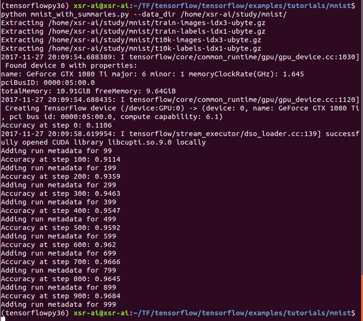
很明显，使用卷积神经网络，准确率大大提高到了0.9684，那么会保存哪些东西呢？

进入到SavedModelBuilder指定的路径“/home/xsr-ai/study/mnist/saved-model”，发现生成了如下东西：

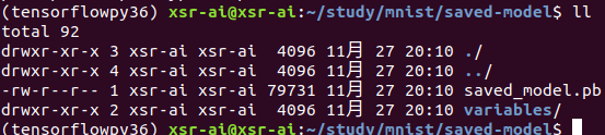
一个pb文件，以及一个variables文件夹，里面存放的是variables.data-00000-of-00001和

variables.index，与save/restore方法比，没有checkpoint检查点文件以及以“.meta”为后缀的元数据文件，但是多了一个pb文件，这是这两种tensorflow保存和恢复模型方法的区别！

 

那么又如何恢复由builder保存的模型呢？我使用如下例子来说明如何使用loader来恢复模型，代码比较简洁，主要是测试恢复模型后，可否正常获取到特定的变量权值：

import tensorflow as tf

with tf.Session() as sess:
  tf.saved_model.loader.load(sess, [tf.saved_model.tag_constants.TRAINING], "/home/xsr-ai/study/mnist/saved-model")
  var = sess.run('layer2/biases/Variable:0')
  print(var)

在jupyter notebook里执行该程序，可得到如下输出：

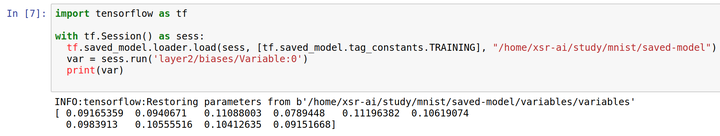
打印出来的layer2/biases/Variable即是模型训练时的最终值，可见，我们保存一个模型后，也是可以恢复然后再进行分析的！