【CVPR2024】Salience DETR: 端到端目标检测计算量减少30%且性能更高!

【CVPR2024】Salience DETR: Enhancing Detection Transformer with Hierarchical Salience Filtering Refinement

机构：西安交通大学、浙江大学

论文地址：https://arxiv.org/abs/2403.16131

代码地址：https://github.com/xiuqhou/Salience-DETR

论文讲解：https://www.bilibili.com/video/BV1sM4m1k7y7

代码讲解：https://www.bilibili.com/video/BV1gt421u79u

本文主要解决DETR方法中计算量高、小物体难检测的问题，考虑到前景比背景信息更重要，文章提出了分层过滤的机制，仅对前景query进行注意力编码，从而降低计算量。并提出了一系列即插即用的query微调模块来加强query之间的信息交互和融合。Salience-DETR相比DINO降低了30%计算量，速度更快，同时性能更高，与Rank-DETR相当。

文章贡献/创新点

• 分析了目标检测存在的两个问题：冗余性和尺寸偏好。
• 提出分层过滤的机制来从特征图和Transformer layer两个层次对query进行过滤，降低计算量。
• 针对过滤后query之间的特征差异，提出三个即插即用的微调模块提升性能。
• 实验验证了所提方法的有效性，相比DINO降低30%计算量但性能更高。

两阶段DETR存在的问题：冗余性和尺寸偏好

主流的高性能DETR采用两阶段的流程：backbone提取多尺度特征图，一阶段Encoder将特征图映射为query，二阶段Decoder筛选最重要的$n$个query进行解码，并通过检测头将其映射为检测结果。文章发现两阶段筛选出的query存在两个问题：

• 冗余性：很多query并没有匹配到物体上，存在冗余性。
• 尺寸偏好：很多query会重复地匹配到大目标上，而有些小目标则匹配不到query，导致小尺寸目标难以被检测到。

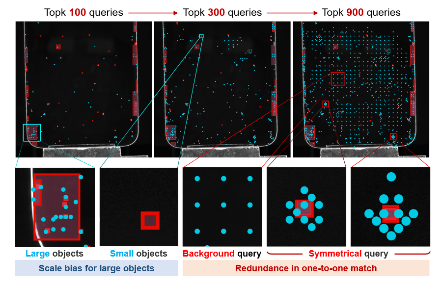
文章对此提出了Salience-DETR，在Encoder中引入了分层过滤机制，在Decoder之前的筛选过程引入了微调机制，来解决这些问题。

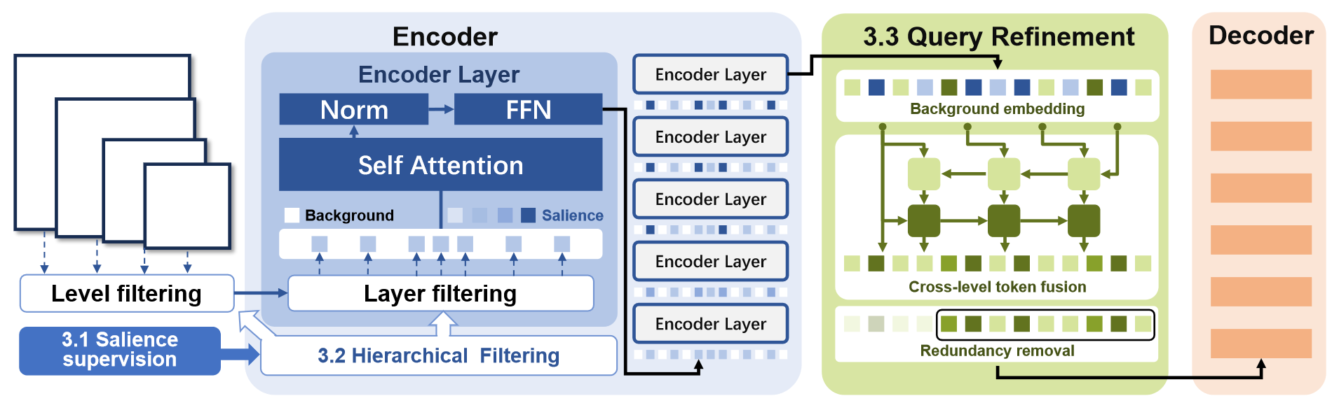
分层过滤机制

Salience-DETR引入了额外的MLP去预测query的显著性分数，仅过滤出最显著的query进行Encoder编码，从而降低计算量。

显著性分数

通常来说，离目标越近的query越重要，且前景比背景重要，中心比边缘重要。已有工作Focus-DETR是将处于背景区域的query分数设为0，前景分数设为1，来强调前景比背景重要。Salience-DETR则进一步让分数随着与物体中心的距离增加而逐渐衰减，接近物体中心的query分数接近1，接近物体边缘的query分数接近0，以强调中心比边缘重要：

$${\theta }_l^{(i,j)}=\{\begin{array}{r}d(\mathbf{c},{\mathcal{D}}_{Bbox}),\mathbf{c}\in {\mathcal{D}}_{Bbox}\\ 0,\mathbf{c}\notin {\mathcal{D}}_{Bbox}\end{array}$$

其中$\mathbf{c}=(x,y)$表示每个query在特征图上的坐标，$\mathbf{c}\in {\mathcal{D}}_{Bbox}$表示处于目标框中的物体。对于处于目标框中的物体，按照如下规则进行衰减：

$$d(\mathbf{c},{\mathcal{D}}_{Bbox})=1-\sqrt{2{\left(\frac{\Delta x}{w}\right)}^2+2{\left(\frac{\Delta y}{h}\right)}^2}$$

其中$\Delta x$和$\Delta y$表示query在横纵坐标上距离物体中心的距离。这样无论目标大小如何，其中心区域总是最显著的，可视化后如下图：

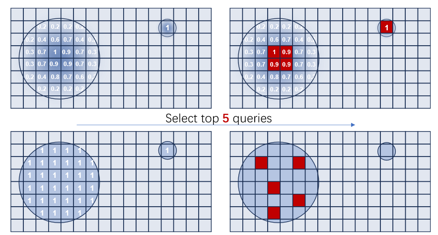
在代码实现中，query会和每个物体中心计算距离delta_x和delta_y，按照上面公式query可以和每个box的都计算出一个显著性confidence_per_box，由于query可能处于多个框的前景区域，代码取最高的框的显著性作为query的显著性，即代码中的mask，最后将背景区域的mask设置为0。

def get_mask_single_level(self, coord_x, coord_y, gt_boxes, level_idx):
    # gt_label: (m,) gt_boxes: (m, 4)
    # coord_x: (h*w, )
    left_border_distance = coord_x[:, None] - gt_boxes[None, :, 0]  # (h*w, m)
    top_border_distance = coord_y[:, None] - gt_boxes[None, :, 1]
    right_border_distance = gt_boxes[None, :, 2] - coord_x[:, None]
    bottom_border_distance = gt_boxes[None, :, 3] - coord_y[:, None]
    border_distances = torch.stack(
        [left_border_distance, top_border_distance, right_border_distance, bottom_border_distance],
        dim=-1,
    )  # [h*w, m, 4]

    # the foreground queries must satisfy two requirements:
    # 1. the quereis located in bounding boxes
    # 2. the distance from queries to the box center match the feature map stride
    min_border_distances = torch.min(border_distances, dim=-1)[0]  # [h*w, m]
    max_border_distances = torch.max(border_distances, dim=-1)[0]
    mask_in_gt_boxes = min_border_distances > 0
    min_limit, max_limit = self.limit_range[level_idx]
    mask_in_level = (max_border_distances > min_limit) & (max_border_distances <= max_limit)
    mask_pos = mask_in_gt_boxes & mask_in_level

    # scale-independent salience confidence
    row_factor = left_border_distance + right_border_distance
    col_factor = top_border_distance + bottom_border_distance
    delta_x = (left_border_distance - right_border_distance) / row_factor
    delta_y = (top_border_distance - bottom_border_distance) / col_factor
    confidence = torch.sqrt(delta_x**2 + delta_y**2) / 2

    confidence_per_box = 1 - confidence
    confidence_per_box[~mask_in_gt_boxes] = 0

    # process positive coordinates
    if confidence_per_box.numel() != 0:
        mask = confidence_per_box.max(-1)[0]
    else:
        mask = torch.zeros(coord_y.shape, device=confidence.device, dtype=confidence.dtype)

    # process negative coordinates
    mask_pos = mask_pos.long().sum(dim=-1) >= 1
    mask[~mask_pos] = 0

    # add noise to add randomness
    mask = (1 - self.noise_scale) * mask + self.noise_scale * torch.rand_like(mask)
    return mask

分层过滤

上面得到的显著性分数作为真值去监督训练MLP，MLP输出每层特征图${\mathbf{f}}_l$对应的显著性分数${\mathbf{s}}_l$，用于对相应的query进行排序和过滤。MLP的流程与Focus-DETR一致，低层特征图在${\mathbf{f}}_{l-1}$会和高一层特征图的预测结果${\mathbf{s}}_l$进行加权，加权后的结果作为MLP的输入，权重${\alpha }_l$作为网络参数自适应去学习。

$${\mathbf{s}}_{l-1}={\mathbf{MLP}}_{\mathbf{F}}({\mathbf{f}}_{l-1}(1+\mathbf{UP}({\alpha }_l\ast {\mathbf{s}}_l)))$$

相应的代码实现如下，由高到低进行预测query的重要性分数，高层分数上采样后得到upsample_score，该分数会和低层特征图level_memory加权，权重self.alpha[level_idx]即${\alpha }_l$，加权后的结果送入enc_mask_predictor网络预测低层query的重要性分数score。

# from high level to low level
batch_size = feat_flatten.shape[0]
selected_score = []
selected_inds = []
salience_score = []
for level_idx in range(spatial_shapes.shape[0] - 1, -1, -1):
    start_index = level_start_index[level_idx]
    end_index = level_start_index[level_idx + 1] if level_idx < spatial_shapes.shape[0] - 1 else None
    level_memory = backbone_output_memory[:, start_index:end_index, :]
    mask = mask_flatten[:, start_index:end_index]
    # update the memory using the higher-level score_prediction
    if level_idx != spatial_shapes.shape[0] - 1:
        upsample_score = torch.nn.functional.interpolate(
            score,
            size=spatial_shapes[level_idx].unbind(),
            mode="bilinear",
            align_corners=True,
        )
        upsample_score = upsample_score.view(batch_size, -1, spatial_shapes[level_idx].prod())
        upsample_score = upsample_score.transpose(1, 2)
        level_memory = level_memory + level_memory * upsample_score * self.alpha[level_idx]
    # predict the foreground score of the current layer
    score = self.enc_mask_predictor(level_memory)
    valid_score = score.squeeze(-1).masked_fill(mask, score.min())
    score = score.transpose(1, 2).view(batch_size, -1, *spatial_shapes[level_idx])

    # get the topk salience index of the current feature map level
    level_score, level_inds = valid_score.topk(level_token_nums[level_idx], dim=1)
    level_inds = level_inds + level_start_index[level_idx]
    salience_score.append(score)
    selected_inds.append(level_inds)
    selected_score.append(level_score)

文章会根据预测得到的${\mathbf{s}}_l$对query进行降序排序，并在特征图层次和编码器层次两个进行过滤，即分层过滤机制。

• 特征图层次：每层特征图仅保留$w_l$比例的query，越高层特征图$w_l$越大，然后将保留的query合并到一起送入Encoder。

• 编码器层次：合并后的query按照合并后的$\mathbf{s}$继续降序排序，在经过每层编码层$t$时，只有其中$w_t$比例的query会进行注意力编码，其他query不做处理：

  $$q_i=\{\begin{array}{rl}\mathrm{Attention}(q_i+po{s}_i,\mathbf{q}+\mathbf{pos},\mathbf{q}),& \text{if}{q}_i\in {\Omega }_t\\ q_i,& \text{if}(q_i\notin {\Omega }_t)\end{array}$$

Query微调机制

文章认为过滤后的query之间存在语义差异，那些经过Transformer编码的query可能具有更强的语义信息，而没有经过处理的query语义信息较弱。因此引入了三个即插即用的微调模块来加强前后景、不同query之间的信息交互和融合。模块的输入和输出都是query。

• 背景嵌入：定义两个embedding分别表示行嵌入${\mathbf{r}}^{(i)}$和列嵌入${\mathbf{c}}^{(j)}$，每个背景query（即从来没有被筛选到得query）会按照其特征图层次$l$、像素坐标$(i,j)$增加相应的行列嵌入，前景则不做处理：

  $${\mathbf{b}}_l^{(i,j)}=\mathrm{Concat}({\mathbf{r}}^{(i)},{\mathbf{c}}^{(j)})$$

  这里其实跟MAE差不多，都是为背景token加上网络自适应学习的embedding。不同之处在于MAE会为所有背景token增加相同的单个embedding，Salience-DETR则是定义了一组行embedding和列embdding，然后根据位置来选择embedding。

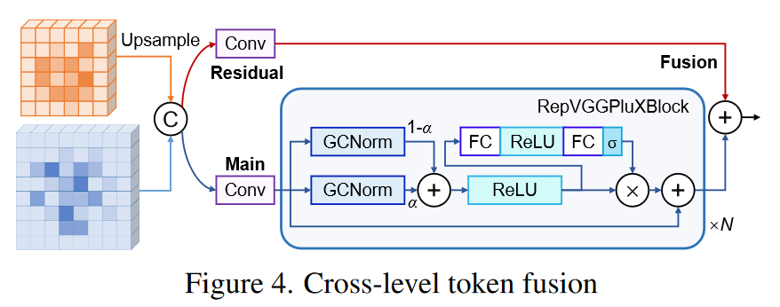
• 跨层融合：增加背景嵌入后，query会使用YOLO中常用的PANet进行多尺度特征融合，只不过将其中的融合模块改进成如下的形式：

  

• 去重：在输入Decoder之前，会去除位置近邻的query来降低重复性。本文以每个query为中心定义了一个3*3的框，然后对框进行NMS，这样如果有query处于3*3网格内，只有其中的1个会被保留。

  $$Bbo{x}_l^{(i,j)}=[i-1,j-1,i+1,j+1]$$

实验结果

从消融实验看，基本每个模块都会提升一些性能，其中微调模块中的背景嵌入和去重并不会增加FLOPs

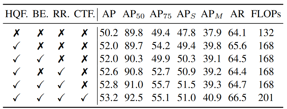
模型性能比DINO和AlignDETR要高，和Stable-DINO和Rank-DETR差不多，优势在于速度快。

Model	backbone	mAP	AP50	AP75	APS	APM	APL	Download
Salience DETR	ResNet50	50.0	67.7	54.2	33.3	54.4	64.4	config / checkpoint
Salience DETR	ConvNeXt-L	54.2	72.4	59.1	38.8	58.3	69.6	config / checkpoint
Salience DETR	Swin-L(IN-22K)	56.5	75.0	61.5	40.2	61.2	72.8	config / checkpoint
Salience DETR	FocalNet-L(IN-22K)	57.3	75.5	62.3	40.9	61.8	74.5	config / checkpoint

24 epoch setting

Model	backbone	mAP	AP50	AP75	APS	APM	APL	Download
Salience DETR	ResNet50	51.2	68.9	55.7	33.9	55.5	65.6	config / checkpoint

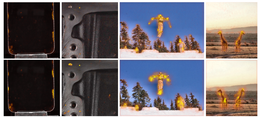
另外一个有意思的点在于，文章虽然只用了检测框标注，但网络预测出的显著性却能够大致匹配到物体轮廓，达到某种程度上分割的效果，也许可以扩展到分割任务。