深度学习6:softmax线性分类器与神经网络分类的性能比较

本文会比较softmax分类与三层神经网络的性能进行比较。

第一步构造数据集：

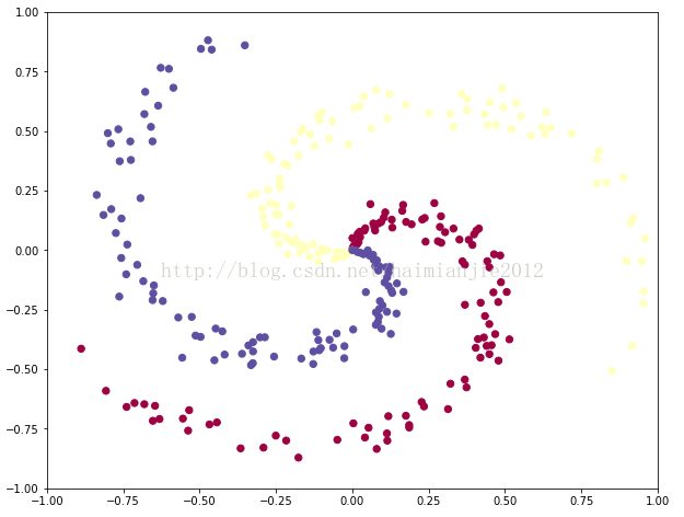
构造数据集源码：（编译环境Jupyter Notebook python3)

import numpy as np
import matplotlib.pyplot as plt

#ubuntu 16.04 sudo pip instal matplotlib

plt.rcParams['figure.figsize'] = (10.0, 8.0) # set default size of plots
plt.rcParams['image.interpolation'] = 'nearest'
plt.rcParams['image.cmap'] = 'gray'

np.random.seed(0)
N = 100 # number of points per class
D = 2 # dimensionality
K = 3 # number of classes
X = np.zeros((N*K,D))
y = np.zeros(N*K, dtype='uint8')
for j in range(K):
  ix = range(N*j,N*(j+1))
  r = np.linspace(0.0,1,N) # radius
  t = np.linspace(j*4,(j+1)*4,N) + np.random.randn(N)*0.2 # theta
  X[ix] = np.c_[r*np.sin(t), r*np.cos(t)]
  y[ix] = j
fig = plt.figure()
plt.scatter(X[:, 0], X[:, 1], c=y, s=40, cmap=plt.cm.Spectral)
plt.xlim([-1,1])
plt.ylim([-1,1])
plt.show()

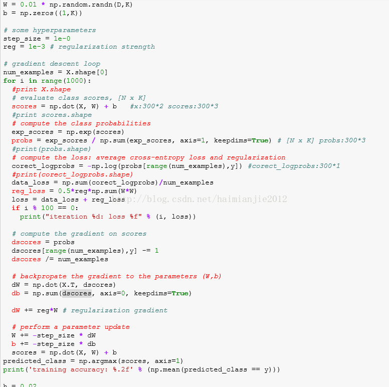
第二步，实现softmax分类器，并分析查看结果：

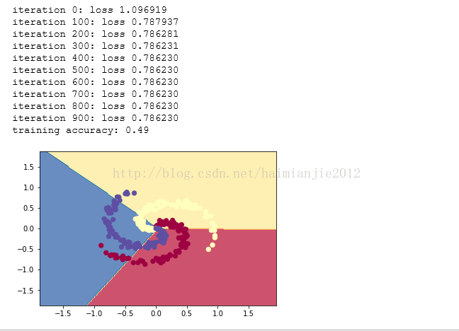
利用优化好的参数W,b构造Z，并绘制分类效果：

softmax分类器的分类效果：

softmax分类器实现源码：编译环境Jupyter Notebook python3

#Train a Linear Classifier
import numpy as np
import matplotlib.pyplot as plt


np.random.seed(0)
N = 100 # number of points per class
D = 2 # dimensionality
K = 3 # number of classes
X = np.zeros((N*K,D))
y = np.zeros(N*K, dtype='uint8')
for j in range(K):
  ix = range(N*j,N*(j+1))
  r = np.linspace(0.0,1,N) # radius
  t = np.linspace(j*4,(j+1)*4,N) + np.random.randn(N)*0.2 # theta
  X[ix] = np.c_[r*np.sin(t), r*np.cos(t)]
  y[ix] = j



W = 0.01 * np.random.randn(D,K)
b = np.zeros((1,K))

# some hyperparameters
step_size = 1e-0
reg = 1e-3 # regularization strength

# gradient descent loop
num_examples = X.shape[0]
for i in range(1000):
  #print X.shape
  # evaluate class scores, [N x K]
  scores = np.dot(X, W) + b   #x:300*2 scores:300*3
  #print scores.shape 
  # compute the class probabilities
  exp_scores = np.exp(scores)
  probs = exp_scores / np.sum(exp_scores, axis=1, keepdims=True) # [N x K] probs:300*3
  #print(probs.shape) 
  # compute the loss: average cross-entropy loss and regularization
  corect_logprobs = -np.log(probs[range(num_examples),y]) #corect_logprobs:300*1
  #print(corect_logprobs.shape) 
  data_loss = np.sum(corect_logprobs)/num_examples
  reg_loss = 0.5*reg*np.sum(W*W)
  loss = data_loss + reg_loss
  if i % 100 == 0:
    print("iteration %d: loss %f" % (i, loss)) 
  
  # compute the gradient on scores
  dscores = probs
  dscores[range(num_examples),y] -= 1
  dscores /= num_examples
  
  # backpropate the gradient to the parameters (W,b)
  dW = np.dot(X.T, dscores)
  db = np.sum(dscores, axis=0, keepdims=True)
  
  dW += reg*W # regularization gradient
  
  # perform a parameter update
  W += -step_size * dW
  b += -step_size * db
  scores = np.dot(X, W) + b
predicted_class = np.argmax(scores, axis=1)
print('training accuracy: %.2f' % (np.mean(predicted_class == y))) 

h = 0.02
x_min, x_max = X[:, 0].min() - 1, X[:, 0].max() + 1
y_min, y_max = X[:, 1].min() - 1, X[:, 1].max() + 1
xx, yy = np.meshgrid(np.arange(x_min, x_max, h),
                     np.arange(y_min, y_max, h))
Z = np.dot(np.c_[xx.ravel(), yy.ravel()], W) + b
Z = np.argmax(Z, axis=1)
Z = Z.reshape(xx.shape)
fig = plt.figure()
plt.contourf(xx, yy, Z, cmap=plt.cm.Spectral, alpha=0.8)
plt.scatter(X[:, 0], X[:, 1], c=y, s=40, cmap=plt.cm.Spectral)
plt.xlim(xx.min(), xx.max())
plt.ylim(yy.min(), yy.max())
plt.show()

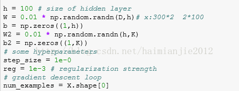
第三步，实现三层神经网络，这次神经网络的激活函数使用relu函数

初始化神经网络参数：

训练网络模型：

测试模型效果，并分析绘制结果：

神经网络模型的测试结果：

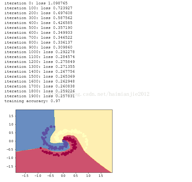
从结果中可以看出，神经网络更能很好地对非线性数据进行分类。

神经网络模型源码：

import numpy as np
import matplotlib.pyplot as plt

np.random.seed(0)
N = 100 # number of points per class
D = 2 # dimensionality
K = 3 # number of classes
X = np.zeros((N*K,D))
y = np.zeros(N*K, dtype='uint8')
for j in range(K):
  ix = range(N*j,N*(j+1))
  r = np.linspace(0.0,1,N) # radius
  t = np.linspace(j*4,(j+1)*4,N) + np.random.randn(N)*0.2 # theta
  X[ix] = np.c_[r*np.sin(t), r*np.cos(t)]
  y[ix] = j
  
h = 100 # size of hidden layer
W = 0.01 * np.random.randn(D,h)# x:300*2  2*100
b = np.zeros((1,h))
W2 = 0.01 * np.random.randn(h,K)
b2 = np.zeros((1,K))

# some hyperparameters
step_size = 1e-0
reg = 1e-3 # regularization strength

# gradient descent loop
num_examples = X.shape[0]
for i in range(2000):
  
  # evaluate class scores, [N x K]
  hidden_layer = np.maximum(0, np.dot(X, W) + b) # note, ReLU activation hidden_layer:300*100
  #print hidden_layer.shape
  scores = np.dot(hidden_layer, W2) + b2  #scores:300*3
  #print scores.shape
  # compute the class probabilities
  exp_scores = np.exp(scores)
  probs = exp_scores / np.sum(exp_scores, axis=1, keepdims=True) # [N x K]
  #print probs.shape
  
  # compute the loss: average cross-entropy loss and regularization
  corect_logprobs = -np.log(probs[range(num_examples),y])
  data_loss = np.sum(corect_logprobs)/num_examples
  reg_loss = 0.5*reg*np.sum(W*W) + 0.5*reg*np.sum(W2*W2)
  loss = data_loss + reg_loss
  if i % 100 == 0:
    print("iteration %d: loss %f" % (i, loss)) 
  
  # compute the gradient on scores
  dscores = probs
  dscores[range(num_examples),y] -= 1
  dscores /= num_examples
  
  # backpropate the gradient to the parameters
  # first backprop into parameters W2 and b2
  dW2 = np.dot(hidden_layer.T, dscores)
  db2 = np.sum(dscores, axis=0, keepdims=True)
  # next backprop into hidden layer
  dhidden = np.dot(dscores, W2.T)
  # backprop the ReLU non-linearity
  dhidden[hidden_layer <= 0] = 0
  # finally into W,b
  dW = np.dot(X.T, dhidden)
  db = np.sum(dhidden, axis=0, keepdims=True)
  
  # add regularization gradient contribution
  dW2 += reg * W2
  dW += reg * W
  
  # perform a parameter update
  W += -step_size * dW
  b += -step_size * db
  W2 += -step_size * dW2
  b2 += -step_size * db2
hidden_layer = np.maximum(0, np.dot(X, W) + b)
scores = np.dot(hidden_layer, W2) + b2
predicted_class = np.argmax(scores, axis=1)
print( 'training accuracy: %.2f' % (np.mean(predicted_class == y)))


h = 0.02
x_min, x_max = X[:, 0].min() - 1, X[:, 0].max() + 1
y_min, y_max = X[:, 1].min() - 1, X[:, 1].max() + 1
xx, yy = np.meshgrid(np.arange(x_min, x_max, h),
                     np.arange(y_min, y_max, h))
Z = np.dot(np.maximum(0, np.dot(np.c_[xx.ravel(), yy.ravel()], W) + b), W2) + b2
Z = np.argmax(Z, axis=1)
Z = Z.reshape(xx.shape)
fig = plt.figure()
plt.contourf(xx, yy, Z, cmap=plt.cm.Spectral, alpha=0.8)
plt.scatter(X[:, 0], X[:, 1], c=y, s=40, cmap=plt.cm.Spectral)
plt.xlim(xx.min(), xx.max())
plt.ylim(yy.min(), yy.max())
plt.show()

更多更好文章，欢迎关注微信公众号：深圳程序媛（updatedaybyday)