


标签(空格分隔): 机器学习
前言:
以斯坦福cs231n课程的python编程任务为主线,展开对该课程主要内容的理解和部分数学推导。
该课程相关笔记参考自知乎-CS231n官方笔记授权翻译总集篇发布
课程材料和事例参考自-cs231n
SVM分类器简介:
SVM-支持向量机(Support Vector Machine),是一个有监督的线性分类器
线性分类器:在本模型中,我们从最简单的函数开始,一个线性映射:
这个公式就是平时最常见到的线性函数,常为一维线性函数(即 W 为一维的)。当这种函数扩展到多维度的情况下时就是我们SVM要面临的情况。首先我们要做的处理是将每个图像数据都拉长为一个长度为D的列向量,大小为 [D * 1] 。其中大小为 [K * D] 的矩阵W和大小为 [K 1] 列向量 b 为该函数的参数。以CIFAR-10为例,CIFAR-10中一个图像的大小等于 [32*32*3] ,含了该图像的所有像素信息,这些信息被拉成为一个 [3072 * 1] 的列向量*, W 大小为 [10*3072] , b 的大小为 [10*1] 。因此,3072个数字(素数值)输入函数,函数输出10个数字(不同分类得到的评分)。参数 W 被称为权重(weights)。 b 被称为偏差向量(bias vector)。
理解线性分类器
线性分类器计算图像中3个颜色通道中所有像素的值与权重的矩阵乘,从而得到分类分值。根据我们对权重设置的值,对于图像中的某些位置的某些颜色,函数表现出的得分即对该点的接受程度。例如对于飞机来说,飞机图片中包含有大量的蓝色天空,白色的云彩以及白色的飞机,那么这个飞机分类器就会在蓝色通道上的权重比较多,而在其他通道上的权重就较少,正如笔记中指出的:

一个将图像映射到分类分值的例子。为了便于可视化,假设图像只有4个像素(都是黑白像素,这里不考虑RGB通道),有3个分类(红色代表猫,绿色代表狗,蓝色代表船,注意,这里的红、绿和蓝3种颜色仅代表分类,和RGB通道没有关系)。首先将图像像素拉伸为一个列向量,与W进行矩阵乘,然后得到各个分类的分值。需要注意的是,这个W一点也不好:猫分类的分值非常低。从上图来看,算法倒是觉得这个图像是一只狗。
现在考虑高维度情况:还是以CIFAR-10为例,CIFAR-10中的图片转化成一个向量(3072维)后,就是一个高维度问题,而一个向量(3色通道转化而来)可以看作是3072维空间中的一个点,而线性分类器就是在高维度空间中的一个超平面,将各个空间点分开。如图所示:

图像空间的示意图。其中每个图像是一个点,有3个分类器。以红色的汽车分类器为例,红线表示空间中汽车分类分数为0的点的集合,红色的箭头表示分值上升的方向。所有红线右边的点的分数值均为正,且线性升高。红线左边的点分值为负,且线性降低。
目标:而我们要做的就是寻找一个W和一个b,使得这个超平面能很好的区分各个类。寻找方法就是不停的改变w和b的值,即不停的旋转平移,直到它使分类的偏差较小。
SVM的组成:
- 图像数据预处理:在上面的例子中,所有图像都是使用的原始像素值(从0到255)。在机器学习中,对于输入的特征做归一化(normalization)是必然的。在图像处理中,每个像素点可以看作是一个简单的特征,在一般使用过程中,我们都先将特征“集中”,即训练集中所有的图像计算出一个平均图像值,然后每个图像都减去这个平均值,这样图像的像素值就大约分布在[-127, 127]之间了,下一个常见步骤是,让所有数值分布的区间变为[-1, 1]。
- 损失函数(loss function):如何评判分类器的偏差就是当前的问题,解决这问题的方法就是损失函数:
Li=∑j≠yimax(0,sj−syi+Δ)
这个函数得到的就是当前分类的偏差值。 -
举例:用一个例子演示公式是如何计算的。假设有3个分类,并且得到了分值s=[13,-7,11]。其中第一个类别是正确类别,即 yi=0 。同时假设 Δ 是10。上面的公式是将所有不正确分类加起来,所以得到两个部分:
Li=max(0,−7−13+10)+max(0,11−13+10)
可以看到第一个部分结果是0,这是因为[-7-13+10]得到的是负数,经过函数处理后得到0。这一对类别分数和标签的损失值是0,这是因为正确分类的得分13与错误分类的得分-7的差为20,高于边界值10。而SVM只关心差距至少要大于10,更大的差值还是算作损失值为0。第二个部分计算[11-13+10]得到8。虽然正确分类的得分比不正确分类的得分要高(13>11),但是比10的边界值还是小了,分差只有2,这就是为什么损失值等于8。简而言之,SVM的损失函数想要正确分类类别的分数比不正确类别分数高,而且至少要高。如果不满足这点,就开始计算损失值。
那么在这次的模型中,我们面对的是线性评分函数(f(x_i,W)=Wx_i),所以我们可以将损失函数的公式稍微改写一下:
Li=∑j≠yimax(0,wTjxi−wTyixi+Δ)
其中w_j是权重W的第j行,被变形为列向量。然而,一旦开始考虑更复杂的评分函数f公式,这样做就不是必须的了。 - 正则化(Regularization):上面损失函数有一个问题。假设有一个数据集和一个权重集W能够正确地分类每个数据(即所有的边界都满足,对于所有的i都有)。问题在于这个W并不唯一:可能有很多相似的W都能正确地分类所有的数据。
-
一个简单的例子:如果W能够正确分类所有数据,即对于每个数据,损失值都是0。那么当时,任何数乘都能使得损失值为0,因为这个变化将所有分值的大小都均等地扩大了,所以它们之间的绝对差值也扩大了。举个例子,如果一个正确分类的分值和举例它最近的错误分类的分值的差距是15,对W乘以2将使得差距变成30。
当然,在没有这种模糊性的情况下我们能很好的控制偏差。而减少这种模糊性的方法是向损失函数增加一个正则化惩罚(regularization penalty)部分。最常用的正则化惩罚是L2范式,L2范式通过对所有参数进行逐元素的平方惩罚来抑制大数值的权重,将其展开完整公式是:
L=1N∑i∑j≠yi[max(0,f(xi;W)j−f(xi;W)yi+Δ)]+λ∑k∑lW2k,l其中,N是训练集的数据量。现在正则化惩罚添加到了损失函数里面,并用超参数来计算其权重。该超参数无法简单确定,需要通过交叉验证来获取,引入了L2惩罚后,SVM们就有了最大边界这一良好性质。(如果感兴趣,可以查看CS229课程)。
SVM实现:
- linear_svm.py
-
#coding:utf-8 import numpy as np from random import shuffle def svm_loss_naive(W, X, y, reg): """ Structured SVM loss function, naive implementation (with loops). Inputs have dimension D, there are C classes, and we operate on minibatches of N examples. Inputs: - W: A numpy array of shape (D, C) containing weights. - X: A numpy array of shape (N, D) containing a minibatch of data. - y: A numpy array of shape (N,) containing training labels; y[i] = c means that X[i] has label c, where 0 <= c < C. - reg: (float) regularization strength Returns a tuple of: - loss as single float - gradient with respect to weights W; an array of same shape as W """ dW = np.zeros(W.shape) # initialize the gradient as zero # compute the loss and the gradient num_classes = W.shape[1] num_train = X.shape[0] loss = 0.0 for i in xrange(num_train): scores = X[i].dot(W) correct_class_score = scores[y[i]] for j in xrange(num_classes): if j == y[i]: continue margin = scores[j] - correct_class_score + 1 # note delta = 1 if margin > 0: loss += margin dW[:, y[i]] += -X[i, :] dW[:, j] += X[i, :] # Right now the loss is a sum over all training examples, but we want it # to be an average instead so we divide by num_train. loss /= num_train dW /= num_train # Add regularization to the loss. loss += reg * np.sum(W * W) dW += reg * W return loss, dW def svm_loss_vectorized(W, X, y, reg): """ Structured SVM loss function, vectorized implementation. Inputs and outputs are the same as svm_loss_naive. """ loss = 0.0 dW = np.zeros(W.shape) # initialize the gradient as zero scores = X.dot(W) num_classes = W.shape[1] num_train = X.shape[0] scores_correct = scores[np.arange(num_train), y] # 1 by N scores_correct = np.reshape(scores_correct, (num_train, -1)) # N by 1 margins = scores - scores_correct + 1 # N by C margins = np.maximum(0,margins) margins[np.arange(num_train), y] = 0 loss += np.sum(margins) / num_train loss += 0.5 * reg * np.sum(W * W) # compute the gradient margins[margins > 0] = 1 row_sum = np.sum(margins, axis=1) # 1 by N margins[np.arange(num_train), y] = -row_sum dW += np.dot(X.T, margins)/num_train + reg * W # D by C return loss, dW - linear_classifier.py
-
#coding:utf-8
import numpy as np
from classifiers.linear_svm import *
from classifiers.softmax import *

class LinearClassifier(object):

  def __init__(self,w=None):
    self.W = w

  def train(self, X, y, learning_rate=1e-3, reg=1e-5, num_iters=100,
            batch_size=200, verbose=False):
    """
    Train this linear classifier using stochastic gradient descent.

    Inputs:
    - X: A numpy array of shape (N, D) containing training data; there are N
      training samples each of dimension D.
    - y: A numpy array of shape (N,) containing training labels; y[i] = c
      means that X[i] has label 0 <= c < C for C classes.
    - learning_rate: (float) learning rate for optimization.
    - reg: (float) regularization strength.
    - num_iters: (integer) number of steps to take when optimizing
    - batch_size: (integer) number of training examples to use at each step.
    - verbose: (boolean) If true, print progress during optimization.

    Outputs:
    A list containing the value of the loss function at each training iteration.
    """
    num_train, dim = X.shape
    num_classes = np.max(y) + 1 # assume y takes values 0...K-1 where K is number of classes
    if self.W is None:
      # lazily initialize W
      self.W = 0.001 * np.random.randn(dim, num_classes)

    # Run stochastic gradient descent to optimize W
    loss_history = []
    for it in xrange(num_iters):
      X_batch = None
      y_batch = None

      sample_index = np.random.choice(num_train, batch_size, replace=False)
      X_batch = X[sample_index, :]   # select the batch sample
      y_batch = y[sample_index]      # select the batch label

      # evaluate loss and gradient
      loss, grad = self.loss(X_batch, y_batch, reg)
      loss_history.append(loss)

      # perform parameter update
      self.W += -learning_rate * grad

      if verbose and it % 100 == 0:
        print 'iteration %d / %d: loss %f' % (it, num_iters, loss)

    return loss_history

  def predict(self, X):
    """
    Use the trained weights of this linear classifier to predict labels for
    data points.

    Inputs:
    - X: D x N array of training data. Each column is a D-dimensional point.

    Returns:
    - y_pred: Predicted labels for the data in X. y_pred is a 1-dimensional
      array of length N, and each element is an integer giving the predicted
      class.
    """
    y_pred = np.zeros(X.shape[1])
    score = X.dot(self.W)
    y_pred = np.argmax(score,axis=1)
    return y_pred

  def loss(self, X_batch, y_batch, reg):
    """
    Compute the loss function and its derivative.
    Subclasses will override this.

    Inputs:
    - X_batch: A numpy array of shape (N, D) containing a minibatch of N
      data points; each point has dimension D.
    - y_batch: A numpy array of shape (N,) containing labels for the minibatch.
    - reg: (float) regularization strength.

    Returns: A tuple containing:
    - loss as a single float
    - gradient with respect to self.W; an array of the same shape as W
    """
    pass


class LinearSVM(LinearClassifier):
  """ A subclass that uses the Multiclass SVM loss function """

  def loss(self, X_batch, y_batch, reg):
    return svm_loss_vectorized(self.W, X_batch, y_batch, reg)


class Softmax(LinearClassifier):
  """ A subclass that uses the Softmax + Cross-entropy loss function """

  def loss(self, X_batch, y_batch, reg):
    return softmax_loss_vectorized(self.W, X_batch, y_batch, reg)
测试:
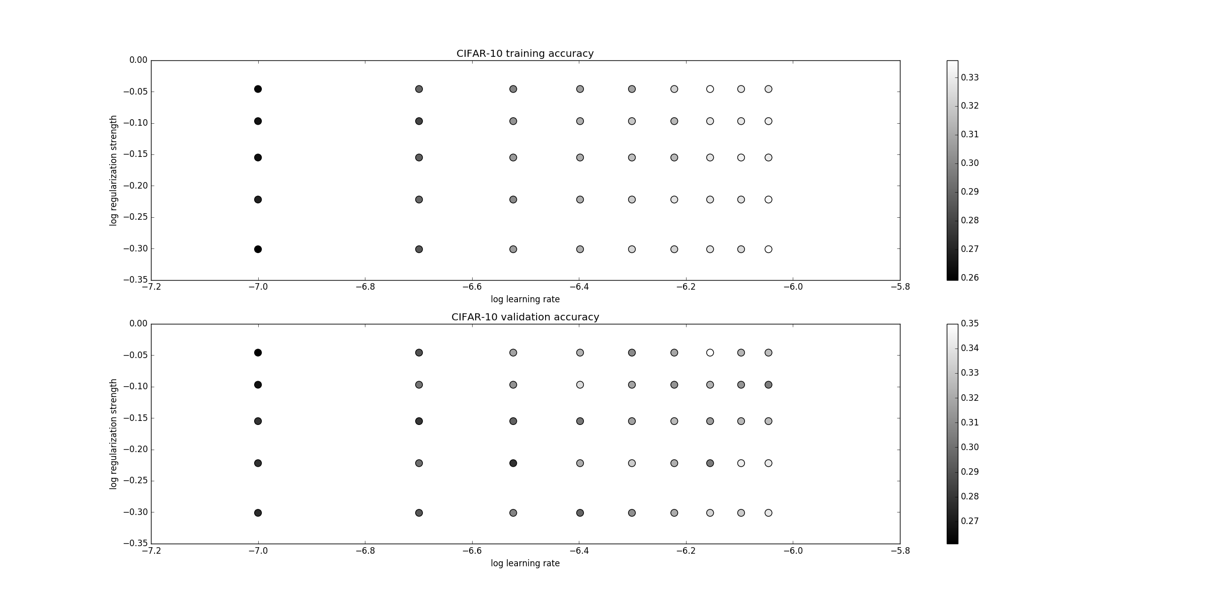
不同参数下SVM10类分类的准确率如下:
总结:
SVM在分类少以及线性的情况下有非常好的分类效果(尤其是二类),在配合PCA的情况下会有更好的结果。


 214
214


 被折叠的 条评论
为什么被折叠?
被折叠的 条评论
为什么被折叠?
 到【灌水乐园】发言


