吴恩达Coursera深度学习课程 deeplearning.ai (5-1) 循环序列模型--编程作业(一)：构建循环神经网络

Part 1: 构建神经网络

欢迎来到本周的第一个作业，这个作业我们将利用numpy实现你的第一个循环神经网络。

循环神经网络(Recurrent Neural Networks: RNN) 因为有”记忆”，所以在自然语言处理(Natural Language Processing) 和其他序列化任务中非常有效。RNN每次读取序列中的一个输入$x^{<t>}$ (比如一个单词), 通过激活函数记住一些信息和上下文，然后传递到下一个实践部。这使得单向RNN可以携带信息想前传播，而双向RNN更是可以携带过去的和未来的上下文信息。

符号说明

• 上标 $^{[l]}$ 表示第l层
• 上标 $^{(i)}$ 表示第i个样本
• 上标 $^{<t>}$ 表示输入x在第t个时间步上的值
• 下标 $_i$ 表示一个向量的第i个维度
• $T_x$ 和 $T_y$ 分别表示输入和输出的时间步数

导包

import numpy as np
from rnn_utils import *

下面是 rnn_utils 中包含的程序：

import numpy as np

def softmax(x):
    e_x = np.exp(x - np.max(x))
    return e_x / e_x.sum(axis=0)


def sigmoid(x):
    return 1 / (1 + np.exp(-x))


def initialize_adam(parameters) :
    """
    Initializes v and s as two python dictionaries with:
                - keys: "dW1", "db1", ..., "dWL", "dbL" 
                - values: numpy arrays of zeros of the same shape as the corresponding gradients/parameters.

    Arguments:
    parameters -- python dictionary containing your parameters.
                    parameters["W" + str(l)] = Wl
                    parameters["b" + str(l)] = bl

    Returns: 
    v -- python dictionary that will contain the exponentially weighted average of the gradient.
                    v["dW" + str(l)] = ...
                    v["db" + str(l)] = ...
    s -- python dictionary that will contain the exponentially weighted average of the squared gradient.
                    s["dW" + str(l)] = ...
                    s["db" + str(l)] = ...

    """

    L = len(parameters) // 2 # number of layers in the neural networks
    v = {}
    s = {}

    # Initialize v, s. Input: "parameters". Outputs: "v, s".
    for l in range(L):
    ### START CODE HERE ### (approx. 4 lines)
        v["dW" + str(l+1)] = np.zeros(parameters["W" + str(l+1)].shape)
        v["db" + str(l+1)] = np.zeros(parameters["b" + str(l+1)].shape)
        s["dW" + str(l+1)] = np.zeros(parameters["W" + str(l+1)].shape)
        s["db" + str(l+1)] = np.zeros(parameters["b" + str(l+1)].shape)
    ### END CODE HERE ###

    return v, s


def update_parameters_with_adam(parameters, grads, v, s, t, learning_rate = 0.01,
                                beta1 = 0.9, beta2 = 0.999,  epsilon = 1e-8):
    """
    Update parameters using Adam

    Arguments:
    parameters -- python dictionary containing your parameters:
                    parameters['W' + str(l)] = Wl
                    parameters['b' + str(l)] = bl
    grads -- python dictionary containing your gradients for each parameters:
                    grads['dW' + str(l)] = dWl
                    grads['db' + str(l)] = dbl
    v -- Adam variable, moving average of the first gradient, python dictionary
    s -- Adam variable, moving average of the squared gradient, python dictionary
    learning_rate -- the learning rate, scalar.
    beta1 -- Exponential decay hyperparameter for the first moment estimates 
    beta2 -- Exponential decay hyperparameter for the second moment estimates 
    epsilon -- hyperparameter preventing division by zero in Adam updates

    Returns:
    parameters -- python dictionary containing your updated parameters 
    v -- Adam variable, moving average of the first gradient, python dictionary
    s -- Adam variable, moving average of the squared gradient, python dictionary
    """

    L = len(parameters) // 2                 # number of layers in the neural networks
    v_corrected = {}                         # Initializing first moment estimate, python dictionary
    s_corrected = {}                         # Initializing second moment estimate, python dictionary

    # Perform Adam update on all parameters
    for l in range(L):
        # Moving average of the gradients. Inputs: "v, grads, beta1". Output: "v".
        ### START CODE HERE ### (approx. 2 lines)
        v["dW" + str(l+1)] = beta1 * v["dW" + str(l+1)] + (1 - beta1) * grads["dW" + str(l+1)] 
        v["db" + str(l+1)] = beta1 * v["db" + str(l+1)] + (1 - beta1) * grads["db" + str(l+1)] 
        ### END CODE HERE ###

        # Compute bias-corrected first moment estimate. Inputs: "v, beta1, t". Output: "v_corrected".
        ### START CODE HERE ### (approx. 2 lines)
        v_corrected["dW" + str(l+1)] = v["dW" + str(l+1)] / (1 - beta1**t)
        v_corrected["db" + str(l+1)] = v["db" + str(l+1)] / (1 - beta1**t)
        ### END CODE HERE ###

        # Moving average of the squared gradients. Inputs: "s, grads, beta2". Output: "s".
        ### START CODE HERE ### (approx. 2 lines)
        s["dW" + str(l+1)] = beta2 * s["dW" + str(l+1)] + (1 - beta2) * (grads["dW" + str(l+1)] ** 2)
        s["db" + str(l+1)] = beta2 * s["db" + str(l+1)] + (1 - beta2) * (grads["db" + str(l+1)] ** 2)
        ### END CODE HERE ###

        # Compute bias-corrected second raw moment estimate. Inputs: "s, beta2, t". Output: "s_corrected".
        ### START CODE HERE ### (approx. 2 lines)
        s_corrected["dW" + str(l+1)] = s["dW" + str(l+1)] / (1 - beta2 ** t)
        s_corrected["db" + str(l+1)] = s["db" + str(l+1)] / (1 - beta2 ** t)
        ### END CODE HERE ###

        # Update parameters. Inputs: "parameters, learning_rate, v_corrected, s_corrected, epsilon". Output: "parameters".
        ### START CODE HERE ### (approx. 2 lines)
        parameters["W" + str(l+1)] = parameters["W" + str(l+1)] - learning_rate * v_corrected["dW" + str(l+1)] / np.sqrt(s_corrected["dW" + str(l+1)] + epsilon)
        parameters["b" + str(l+1)] = parameters["b" + str(l+1)] - learning_rate * v_corrected["db" + str(l+1)] / np.sqrt(s_corrected["db" + str(l+1)] + epsilon)
        ### END CODE HERE ###

    return parameters, v, s

1 基本循环神经网络的前向传播

基本的RNN结构如下：(这里Tx = Ty)

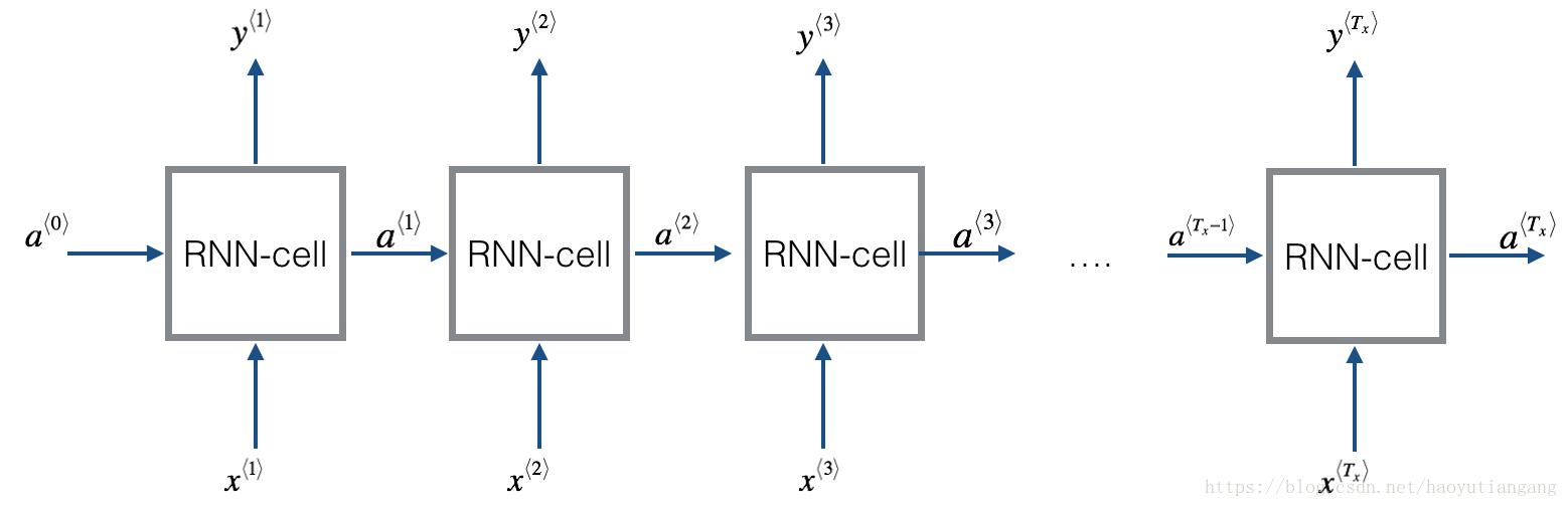
实现循环神经网络

• 实现 RNN 单时间步运算
• 按时间循环Tx的每个时间步运算

1.1 RNN 单元

一个循环神经网络可以看成是单个RNN单元的重复。首先我们将实现一个单时间步的RNN单元的计算，下图描述了单步RNN 的操作。

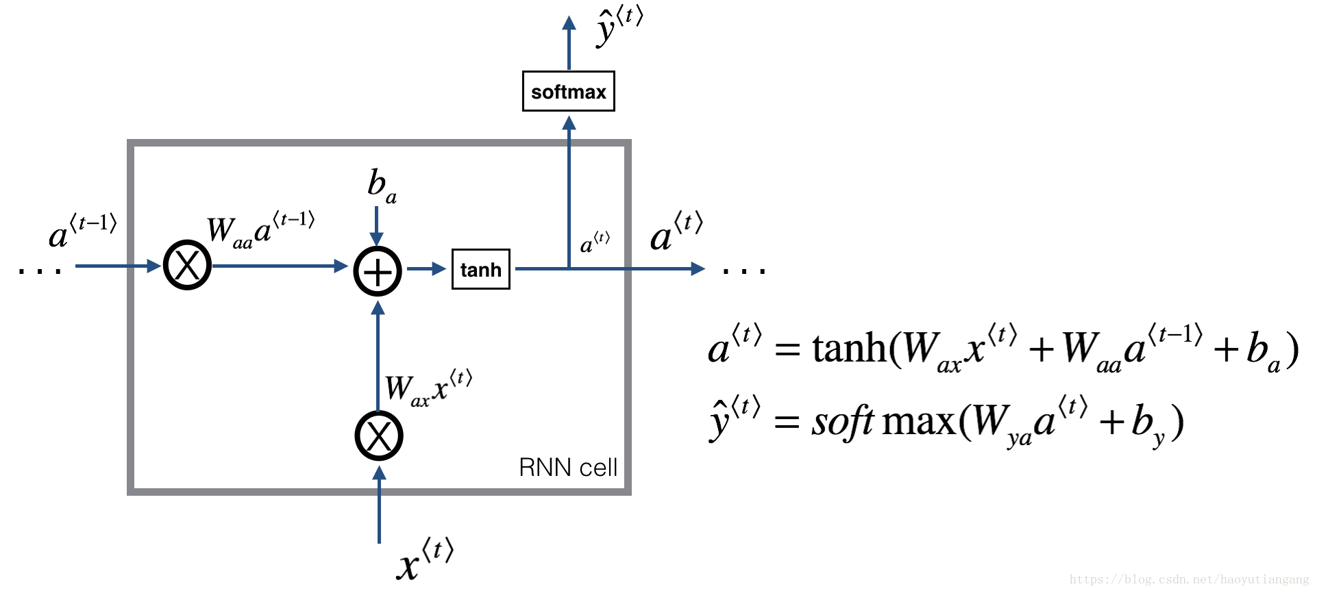
练习：实现上图描述的单步RNN单元

1. 利用tanh激活函数计算隐藏层的状态
   $$a^{\langle t \rangle} = \tanh(W_{aa} a^{\langle t-1 \rangle} + W_{ax} x^{\langle t \rangle} + b_a)$$
2. 使用新的隐藏层状态$a^{<t>}$ 计算预测值$y_{hat}$ （已提供函数softmax）
   $$\hat{y}^{\langle t \rangle} = softmax(W_{ya} a^{\langle t \rangle} + b_y)$$
3. 在cache中存储参数
   $$(a^{\langle t \rangle}, a^{\langle t-1 \rangle}, x^{\langle t \rangle}, parameters)$$
4. 返回 $a^{<t>}$, $y^{<t>}$ 和 cache

我们的输入是m个向量。所以：$x^{<t>}$ 维度：($n_x$, m) ; $a^{<t>}$ 维度：($n_a$, m)

# GRADED FUNCTION: rnn_cell_forward

def rnn_cell_forward(xt, a_prev, parameters):
    """
    Implements a single forward step of the RNN-cell as described in Figure (2)

    Arguments:
    xt -- your input data at timestep "t", numpy array of shape (n_x, m).
    a_prev -- Hidden state at timestep "t-1", numpy array of shape (n_a, m)
    parameters -- python dictionary containing:
                        Wax -- Weight matrix multiplying the input, numpy array of shape (n_a, n_x)
                        Waa -- Weight matrix multiplying the hidden state, numpy array of shape (n_a, n_a)
                        Wya -- Weight matrix relating the hidden-state to the output, numpy array of shape (n_y, n_a)
                        ba --  Bias, numpy array of shape (n_a, 1)
                        by -- Bias relating the hidden-state to the output, numpy array of shape (n_y, 1)
    Returns:
    a_next -- next hidden state, of shape (n_a, m)
    yt_pred -- prediction at timestep "t", numpy array of shape (n_y, m)
    cache -- tuple of values needed for the backward pass, contains (a_next, a_prev, xt, parameters)
    """

    # Retrieve parameters from "parameters"
    Wax = parameters["Wax"]
    Waa = parameters["Waa"]
    Wya = parameters["Wya"]
    ba = parameters["ba"]
    by = parameters["by"]

    ### START CODE HERE ### (≈2 lines)
    # compute next activation state using the formula given above
    a_next = np.tanh(np.dot(Waa, a_prev) + np.dot(Wax, xt) + ba)
    # compute output of the current cell using the formula given above
    yt_pred = softmax(np.dot(Wya, a_next) + by) 
    ### END CODE HERE ###

    # store values you need for backward propagation in cache
    cache = (a_next, a_prev, xt, parameters)

    return a_next, yt_pred, cache

#########################################################

np.random.seed(1)
xt = np.random.randn(3,10)
a_prev = np.random.randn(5,10)
Waa = np.random.randn(5,5)
Wax = np.random.randn(5,3)
Wya = np.random.randn(2,5)
ba = np.random.randn(5,1)
by = np.random.randn(2,1)
parameters = {
  "Waa": Waa, "Wax": Wax, "Wya": Wya, "ba": ba, "by": by}

a_next, yt_pred, cache = rnn_cell_forward(xt, a_prev, parameters)
print("a_next[4] = ", a_next[4])
print("a_next.shape = ", a_next.shape)
print("yt_pred[1] =", yt_pred[1])
print("yt_pred.shape = ", yt_pred.shape)

# a_next[4] =  [ 0.59584544  0.18141802  0.61311866  0.99808218  0.85016201  # 0.99980978
#  -0.18887155  0.99815551  0.6531151   0.82872037]
# a_next.shape =  (5, 10)
# yt_pred[1] = [ 0.9888161   0.01682021  0.21140899  0.36817467  0.98988387  # 0.88945212
#   0.36920224  0.9966312   0.9982559   0.17746526]
# yt_pred.shape =  (2, 10)

期待输出

key	value
a_next[4]:	[ 0.59584544 0.18141802 0.61311866 0.99808218 0.85016201 0.99980978 -0.18887155 0.99815551 0.6531151 0.82872037]
a_next.shape:	(5, 10)
yt[1]:	[ 0.9888161 0.01682021 0.21140899 0.36817467 0.98988387 0.88945212 0.36920224 0.9966312 0.9982559 0.17746526]
yt.shape:	(2, 10)

1.2 RNN 前向传播

比如输入有10个时间步，则依次将单元RNN相连，每个单元的输入来自上层的$a^{<t-1>}$和本层的$x^{<t>}$，输出$a^{<t>}$和$y_{hat}^{<t>}$。

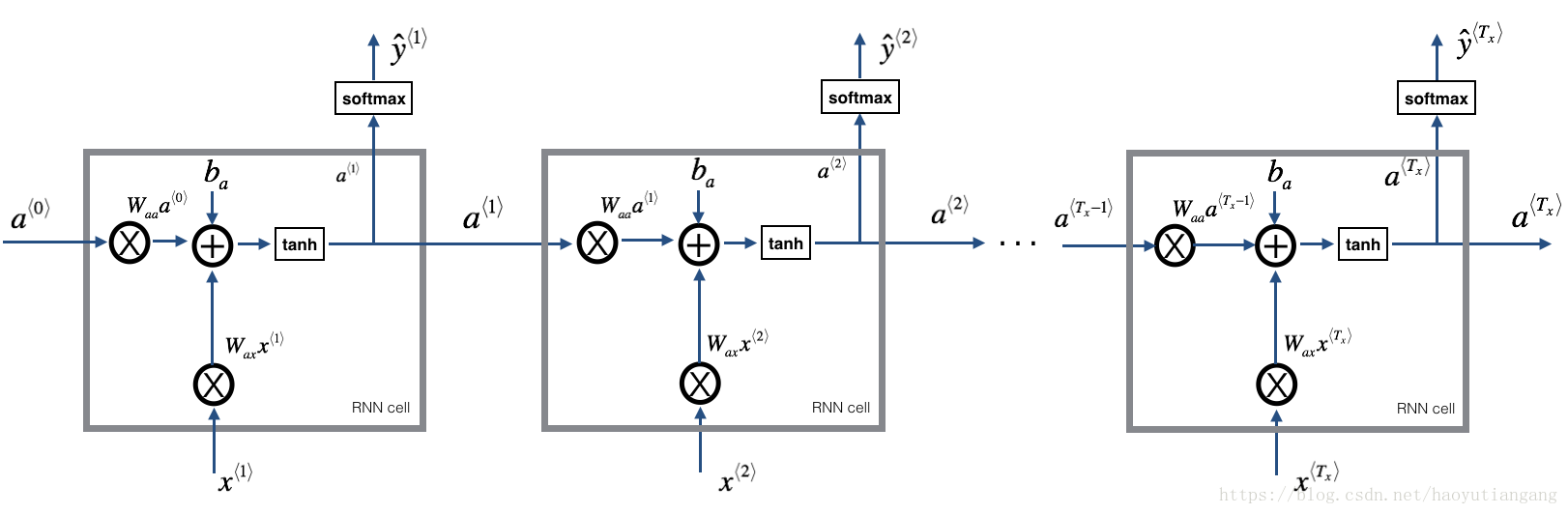
练习：实现上图描述的RNN 的前向传播

1. 创建一个0值向量a, 用来存储RNN计算的所有隐藏状态
2. 初始化”next”隐藏层状态 a0