Chatper 5: Pretraining on Unlabeled Data-CSDN博客

本文链接：https://blog.csdn.net/hbkybkzw/article/details/145213593

文章目录

5 Pretraining on Unlabeled Data

5 Pretraining on Unlabeled Data

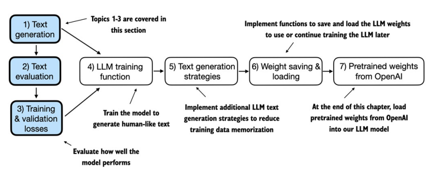
本章节包含：
1. 计算训练集和验证集损失：用于评估训练期间 LLM 生成文本的质量。
2. 实现训练函数并对 LLM 进行预训练：通过编写训练函数，完成 LLM 的预训练过程。
3. 保存和加载模型权重：以便在需要时继续训练 LLM。
4. 加载 OpenAI 的预训练权重：将 OpenAI 的预训练权重加载到模型中，以加速训练或直接使用。
本章节的重点是实现训练功能并对LLM进行预训练。

LLM 开发的三个主要阶段包括：
1. 编码 LLM：实现模型架构和核心组件。
2. 预训练 LLM：在通用文本数据集上训练模型，使其学习语言的基本规律。
3. 微调 LLM：在带标签的数据集上进一步训练，使模型适应特定任务。
本章重点在于 预训练 LLM，涵盖以下内容：
- 实现训练代码
- 评估生成文本的质量（通过计算训练集和验证集损失）
- 保存和加载模型权重
- 加载 OpenAI 的预训练权重，为后续微调提供基础
关键概念
- 权重（Weights）：模型的可训练参数，存储在 PyTorch 的线性层等模块中，可通过 .weight 属性或 model.parameters() 方法访问。
- 模型评估：通过基本技术衡量生成文本的质量，是优化训练过程的必要步骤。
本章为后续章节的微调和优化奠定了基础。

5.1 Evaluating generative text models

本节主要内容如下图 1,2,3
1. 简要回顾一下使用上一章的代码初始化 GPT 模型的内容
2. 讨论 LLMs 的基本评估指标
3. 将评估指标应用于一个训练和验证数据集

5.1.1 Using GPT to generate text

我们使用之前章节的代码初始化一个 GPT 模型
```
import torch
from previous_chapters import GPTModel

GPT_CONFIG_124M = {
    "vocab_size": 50257,   # Vocabulary size
    "context_length": 256, # Shortened context length (orig: 1024)
    "emb_dim": 768,        # Embedding dimension
    "n_heads": 12,         # Number of attention heads
    "n_layers": 12,        # Number of layers
    "drop_rate": 0.1,      # Dropout rate
    "qkv_bias": False      # Query-key-value bias
}

torch.manual_seed(123)
model = GPTModel(GPT_CONFIG_124M)
model.eval();  # Disable dropout during inference
```
需要注意以下几点

这段内容主要介绍了大语言模型（LLMs）训练及相关设置的一些要点：
1. 随机失活（dropout）：上文使用了 0.1 的随机失活，但如今训练 LLMs 时不使用随机失活较为常见
2. 偏置向量设置：现代 LLMs 在 nn.Linear 层处理查询、键和值矩阵时，不像早期 GPT 模型那样使用偏置向量，通过设置 “qkv_bias”: false 实现。
3. 上下文长度（context_length）调整： - 为降低训练模型的计算资源需求，将上下文长度设为 256 个词元，而原始 1.24 亿参数的 GPT - 2 模型使用 1024 个词元。 - 这样做是为方便在笔记本电脑上理解和运行代码示例。

接下来，我们将使用上一章中的 generate_text_simple 函数来生成文本，此外，我们定义了两个便捷函数 text_to_token_ids 和 token_ids_to_text，用于在词元（token）表示和文本表示之间进行转换。

上图展示了使用 GPT 模型的一个三步文本生成过程

tokenizer 将输入的文本转换为 token ids
模型接受 token ids 并生成对应的对数几率(logits)，他们是表示词汇表中每个词元概率分布的向量。
将对数几率转换为 token ids,tokenizer 将其解码为人类可读的文本。

代码如下

import tiktoken
from previous_chapters import generate_text_simple

def text_to_token_ids(text, tokenizer):
    encoded = tokenizer.encode(text, allowed_special={'<|endoftext|>'})
    encoded_tensor = torch.tensor(encoded).unsqueeze(0) # add batch dimension
    return encoded_tensor

def token_ids_to_text(token_ids, tokenizer):
    flat = token_ids.squeeze(0) # remove batch dimension
    return tokenizer.decode(flat.tolist())

start_context = "Every effort moves you"
tokenizer = tiktoken.get_encoding("gpt2")

# text to token_id
input_ids = text_to_token_ids(start_context, tokenizer)
print("Input ids:\n", input_ids)

token_ids = generate_text_simple(
    model=model,
    idx=input_ids,
    max_new_tokens=10,
    context_size=GPT_CONFIG_124M["context_length"]
)
print("Generated token ids:\n", token_ids)

# token_id to text
output_text = token_ids_to_text(token_ids, tokenizer)
print("Gentrated text:\n", output_text)


"""输出如下"""
Input ids:
 tensor([[6109, 3626, 6100,  345]])

Generated token ids:
 tensor([[ 6109,  3626,  6100,   345, 34245,  5139,  2492, 25405, 17434, 17853,
          5308,  3398, 13174, 43071]])

Gentrated text:
  Every effort moves you rentingetic wasnم refres RexMeCHicular stren

基于输出可知模型因未经过训练尚未生成连贯文本，为定义文本“连贯”或“高质量”的标准，需实施数值方法评估生成内容。

5.1.2 Calculating the text generation loss: cross-entropy and perplexity

本节借助计算文本生成损失，探究对训练中生成文本质量进行量化评估的技术。为让相关概念清晰且实用，我们会以实际示例逐步展开讲解。开篇先简要回顾第2章的数据加载方式以及第4章利用 generate_text_simple 函数生成文本的方法。
假设我们有一个inputs张量，其中包含2个训练示例（行）的词元ID（token IDs）。与inputs相对应，targets包含我们希望模型生成的所需词元ID。
```
inputs = torch.tensor([[16833, 3626, 6100],   # ["every effort moves",
                       [40,    1107, 588]])   #  "I really like"]

targets = torch.tensor([[3626, 6100, 345  ],  # [" effort moves you",
                        [1107,  588, 11311]]) #  " really like chocolate"]
```
请注意，如我们在第2章实现数据加载器时所解释的，targets是inputs偏移1个位置后的结果。
```
with torch.no_grad():
    logits = model(inputs)

probas = torch.softmax(logits, dim=-1) # Probability of each token in vocabulary
print(probas.shape) # Shape: (batch_size, num_tokens, vocab_size)

"""输出"""
torch.Size([2, 3, 50257])
```
将inputs输入模型可得两个各由3个词元组成的输入示例的对数几率向量，每个词元是与词汇表大小对应的50,257维向量，应用softmax函数能把该对数几率张量转为同维度的概率得分张量。第一个数字 2 对应于输入中的两个示例（行），也称为批量大小。第二个数字 3 对应于每个输入（行）中的标记数量。最后，最后一个数字对应于嵌入维数，该维数由词汇量决定。

上图仅仅使用一个小的 7 个标记词汇来概述文本生成。对于左侧所示的 3 个输入标记中的每一个，我们计算一个向量，其中包含与词汇表中每个标记相对应的概率分数。每个向量中最高概率得分的索引位置代表最有可能的下一个令牌ID。这些与最高概率分数相关联的令牌 ID 被选择并映射回表示模型生成的文本的文本。
```
token_ids = torch.argmax(probas, dim=-1, keepdim=True)
print("Token IDs:\n", token_ids)

"""输出"""
Token IDs:
 tensor([[[16657],
         [  339],
         [42826]],

        [[49906],
         [29669],
         [41751]]])
```
如前一章所讨论，我们可应用argmax函数将概率得分转换为预测tokenID，鉴于上述softmax函数为每个token生成一个50,257维向量，argmax函数会返回该向量中概率得分最高的位置作为给定token的预测tokenID，又因我们有2个各含3个token的输入批次，故得到一个2×3的预测tokenID矩阵。
如果我们对这些token进行解码，就会发现它们与我们希望模型预测的 token（即目标 token）有很大差异：
```
print(f"Targets batch 1: {token_ids_to_text(targets[0], tokenizer)}")
print(f"Outputs batch 1: {token_ids_to_text(token_ids[0].flatten(), tokenizer)}")

"""输出"""
Targets batch 1:  effort moves you
Outputs batch 1:  Armed heNetflix
```
这是因为模型尚未经过训练，所以为了训练模型，我们需要知道它与正确预测（目标）之间的差距有多大。

当然，上图将所有内容呈现在一张图中展示了一个仅包含7个词元的精简词汇表的softmax概率，这意味着起始随机值会在1/7（约等于0.14）左右波动，而我们用于GPT - 2模型的词汇表有50,257个词元，大部分初始概率会在0.00002左右波动。

对于两个输入文本中的每一个，我们可以通过以下代码打印与目标标记对应的初始softmax概率分数：
```
text_idx = 0
target_probas_1 = probas[text_idx, [0, 1, 2], targets[text_idx]]
print("Text 1:", target_probas_1)

text_idx = 1
target_probas_2 = probas[text_idx, [0, 1, 2], targets[text_idx]]
print("Text 2:", target_probas_2)

"""输出"""
Text 1: tensor([7.4541e-05, 3.1061e-05, 1.1563e-05])
Text 2: tensor([1.0337e-05, 5.6776e-05, 4.7559e-06])
```
我们计算两个示例批次（target_probas_1 和 target_probas_2）的概率分数的损失
```
# Compute logarithm of all token probabilities
log_probas = torch.log(torch.cat((target_probas_1, target_probas_2)))
print(log_probas)

"""输出"""
tensor([ -9.5042, -10.3796, -11.3677, -11.4798,  -9.7764, -12.2561])
```
```
# Calculate the average probability for each token
avg_log_probas = torch.mean(log_probas)
print(avg_log_probas)

"""输出"""
tensor(-10.7940)
```
目标是通过优化模型权重，使这个平均对数概率尽可能大。由于对数的性质，其最大可能值位置为0，而我们目前离0还很远。在深度学习中，标准做法不是最大化平均对数概率，而是最小化平均对数概率的负值。就我们的情况而言，不是要将 -10.7722 最大化使其趋近于0，而是在深度学习中，我们会将 10.7722 最小化，使其趋近于0。-10.7722 的负值，即 10.7722，在深度学习中也被称为交叉熵损失。
```
neg_avg_log_probas = avg_log_probas * -1
print(neg_avg_log_probas)

"""输出"""
tensor(10.7940)
```
PyTorch已经实现了一个cross_entropy函数，该函数可以执行前面提到的步骤。

在应用cross_entropy函数之前，让我们先检查一下对数几率（logits）和目标（targets）的形状。
```
# Logits have shape (batch_size, num_tokens, vocab_size)
print("Logits shape:", logits.shape)

# Targets have shape (batch_size, num_tokens)
print("Targets shape:", targets.shape)

"""输出"""
Logits shape: torch.Size([2, 3, 50257])
Targets shape: torch.Size([2, 3])
```
logits 张量具有三个维度：批量大小、标记数量和词汇量大小。目标张量有两个维度：批量大小和标记数量。

对于PyTorch中的cross_entropy函数，我们希望通过在批次维度上合并这些张量来将它们展平：
```
logits_flat = logits.flatten(0, 1)
targets_flat = targets.flatten()

print("Flattened logits:", logits_flat.shape)
print("Flattened targets:", targets_flat.shape)

"""输出"""
Flattened logits: torch.Size([6, 50257])
Flattened targets: torch.Size([6])
```
请注意，目标值是token ID，它们同时也代表了我们希望在对数几率张量中最大化的索引位置，而PyTorch中的cross_entropy函数会自动在内部对对数几率中那些需要最大化的 token索引应用softmax函数并进行对数概率计算。
```
loss = torch.nn.functional.cross_entropy(logits_flat, targets_flat)
print(loss)

"""输出"""
tensor(10.7940)
```
与交叉熵损失相关的一个概念是大语言模型（LLM）的困惑度。困惑度就是交叉熵损失的指数值。
```
perplexity = torch.exp(loss)
print(perplexity)

"""输出"""
tensor(48725.8203)
```
困惑度（Perplexity）衡量的是模型预测的概率分布与数据集中单词的实际分布的匹配程度。与损失（loss）类似，困惑度越低表明模型的预测越接近实际分布。

困惑度可以通过公式 perplexity = torch.exp (loss) 来计算，将其应用于之前计算出的损失时，返回的结果是 tensor (47678.8633)。

困惑度通常被认为比原始损失值更具可解释性，因为它表示在每一步中模型不确定的有效词汇表大小。在给定的示例中，这意味着模型不确定要从词汇表中的 47678 个单词或词元（tokens）中生成哪一个作为下一个词元。

5.1.3 Calculating the training and validation set losses

我们使用一个相对较小的数据集来训练大语言模型（LLM）（实际上，仅仅是一篇短篇小说）。

原因如下：
- 你无需合适的图形处理器（GPU），就能在笔记本电脑上几分钟内运行代码示例。
- 训练完成得相对较快（只需几分钟而非数周），这对于教学目的很有好处。
- 我们使用的文本来自公有领域，因此可以将其包含在这个 GitHub 代码库中，而不会侵犯任何使用权，也不会使代码库规模过大。
例如，Llama 2 7B 在 2 万亿个词元上进行训练，需要在 A100 GPU 上花费 184,320 GPU 小时。
- 在撰写本文时，亚马逊云服务（AWS）上一台配备 8 个 A100 的云服务器每小时成本约为 30 美元。
- 因此，通过粗略计算，训练这个大语言模型的成本为 184,320÷8×30 美元 = 690,000 美元。

接下来，我们将数据集分为训练集和验证集，并使用第 2 章中的数据加载器来准备用于 LLM 训练的批次。

import os
import urllib.request

file_path = "the-verdict.txt"
url = "https://raw.githubusercontent.com/rasbt/LLMs-from-scratch/main/ch02/01_main-chapter-code/the-verdict.txt"

if not os.path.exists(file_path):
    with urllib.request.urlopen(url) as response:
        text_data = response.read().decode('utf-8')
    with open(file_path, "w", encoding="utf-8") as file:
        file.write(text_data)
else:
    with open(file_path, "r", encoding="utf-8") as file:
        text_data = file.read()

通过打印前100个词和后100个词来快速检查文本是否加载正常。

# First 100 characters
print(text_data[:99])

# Last 100 characters
print(text_data[-99:])

"""输出"""
I HAD always thought Jack Gisburn rather a cheap genius--though a good fellow enough--so it was no 

it for me! The Strouds stand alone, and happen once--but there's no exterminating our kind of art."

total_characters = len(text_data)
total_tokens = len(tokenizer.encode(text_data))

print("Characters:", total_characters)
print("Tokens:", total_tokens)

"""输出"""
Characters: 20479
Tokens: 5145

这段文本仅有 5145 个token

接下来，为训练LLM，我们将数据集划分为训练集和验证集，用第2章的数据加载器准备批次数据，出于可视化目的下图假设 max_length = 6，但训练加载器中 max_length 设为LLM支持的上下文长度，且下图仅展示输入词元，因训练LLM是预测文本下一个单词，所以目标与输入类似只是偏移一个位置。

设置 train_ratio ，使用 90% 数据训练，剩下的 10% 作为训练期间模型评估的验证数据

from previous_chapters import create_dataloader_v1

# Train/validation ratio
train_ratio = 0.90
split_idx = int(train_ratio * len(text_data))
train_data = text_data[:split_idx]
val_data = text_data[split_idx:]


torch.manual_seed(123)

train_loader = create_dataloader_v1(
    train_data,
    batch_size=2,
    max_length=GPT_CONFIG_124M["context_length"],
    stride=GPT_CONFIG_124M["context_length"],
    drop_last=True,
    shuffle=True,
    num_workers=0
)

val_loader = create_dataloader_v1(
    val_data,
    batch_size=2,
    max_length=GPT_CONFIG_124M["context_length"],
    stride=GPT_CONFIG_124M["context_length"],
    drop_last=False,
    shuffle=False,
    num_workers=0
)

# Sanity check

if total_tokens * (train_ratio) < GPT_CONFIG_124M["context_length"]:
    print("Not enough tokens for the training loader. "
          "Try to lower the `GPT_CONFIG_124M['context_length']` or "
          "increase the `training_ratio`")

if total_tokens * (1-train_ratio) < GPT_CONFIG_124M["context_length"]:
    print("Not enough tokens for the validation loader. "
          "Try to lower the `GPT_CONFIG_124M['context_length']` or "
          "decrease the `training_ratio`")

检查下数据是否加载正确(可选)

print("Train loader:")
for x, y in train_loader:
    print(x.shape, y.shape)

print("\nValidation loader:")
for x, y in val_loader:
    print(x.shape, y.shape)
    
"""输出"""
Train loader:
torch.Size([2, 256]) torch.Size([2, 256])
torch.Size([2, 256]) torch.Size([2, 256])
torch.Size([2, 256]) torch.Size([2, 256])
torch.Size([2, 256]) torch.Size([2, 256])
torch.Size([2, 256]) torch.Size([2, 256])
torch.Size([2, 256]) torch.Size([2, 256])
torch.Size([2, 256]) torch.Size([2, 256])
torch.Size([2, 256]) torch.Size([2, 256])
torch.Size([2, 256]) torch.Size([2, 256])

Validation loader:
torch.Size([2, 256]) torch.Size([2, 256])

确认 token 大小在预期的范围内（可选）

train_tokens = 0
for input_batch, target_batch in train_loader:
    train_tokens += input_batch.numel()

val_tokens = 0
for input_batch, target_batch in val_loader:
    val_tokens += input_batch.numel()

print("Training tokens:", train_tokens)
print("Validation tokens:", val_tokens)
print("All tokens:", train_tokens + val_tokens)

"""输出"""
Training tokens: 4608
Validation tokens: 512
All tokens: 5120

接下来，我们实现两个实函数

用于计算给定批次的交叉熵损失。
用于计算数据加载器中用户指定数量批次的损失。

def calc_loss_batch(input_batch, target_batch, model, device):
    input_batch, target_batch = input_batch.to(device), target_batch.to(device)
    logits = model(input_batch)
    loss = torch.nn.functional.cross_entropy(logits.flatten(0, 1), target_batch.flatten())
    return loss


def calc_loss_loader(data_loader, model, device, num_batches=None):
    total_loss = 0.
    if len(data_loader) == 0:
        return float("nan")
    elif num_batches is None:
        num_batches = len(data_loader)
    else:
        # Reduce the number of batches to match the total number of batches in the data loader
        # if num_batches exceeds the number of batches in the data loader
        num_batches = min(num_batches, len(data_loader))
    for i, (input_batch, target_batch) in enumerate(data_loader):
        if i < num_batches:
            loss = calc_loss_batch(input_batch, target_batch, model, device)
            total_loss += loss.item()
        else:
            break
    return total_loss / num_batches

默认情况下， calc_loss_batch 函数会迭代给定数据加载器中的所有批次，将损失累积到total_loss 变量中，然后计算总批次数的损失并求平均值。或者，我们可以通过 num_batches 指定较小的批次数，以加快模型训练期间的评估速度。

若机器配备支持 CUDA 的 GPU，大语言模型（LLM）无需更改代码即可在该 GPU 上训练，且通过 “device” 设置，能保证数据加载到与大语言模型（LLM）相同的设备上。

device = torch.device("cuda" if torch.cuda.is_available() else "cpu")

# Note:
# Uncommenting the following lines will allow the code to run on Apple Silicon chips, if applicable,
# which is approximately 2x faster than on an Apple CPU (as measured on an M3 MacBook Air).
# However, the resulting loss values may be slightly different.

#if torch.cuda.is_available():
#    device = torch.device("cuda")
#elif torch.backends.mps.is_available():
#    device = torch.device("mps")
#else:
#    device = torch.device("cpu")
#
# print(f"Using {device} device.")


model.to(device) # no assignment model = model.to(device) necessary for nn.Module classes


torch.manual_seed(123) # For reproducibility due to the shuffling in the data loader

with torch.no_grad(): # Disable gradient tracking for efficiency because we are not training, yet
    train_loss = calc_loss_loader(train_loader, model, device)
    val_loss = calc_loss_loader(val_loader, model, device)

print("Training loss:", train_loss)
print("Validation loss:", val_loss)

"""输出"""
device = torch.device("cuda" if torch.cuda.is_available() else "cpu")

# Note:
# Uncommenting the following lines will allow the code to run on Apple Silicon chips, if applicable,
# which is approximately 2x faster than on an Apple CPU (as measured on an M3 MacBook Air).
# However, the resulting loss values may be slightly different.

#if torch.cuda.is_available():
#    device = torch.device("cuda")
#elif torch.backends.mps.is_available():
#    device = torch.device("mps")
#else:
#    device = torch.device("cpu")
#
# print(f"Using {device} device.")


model.to(device) # no assignment model = model.to(device) necessary for nn.Module classes


torch.manual_seed(123) # For reproducibility due to the shuffling in the data loader

with torch.no_grad(): # Disable gradient tracking for efficiency because we are not training, yet
    train_loss = calc_loss_loader(train_loader, model, device)
    val_loss = calc_loss_loader(val_loader, model, device)

print("Training loss:", train_loss)
print("Validation loss:", val_loss)

由于模型尚未训练，损失值相对较高。为了进行比较，如果模型学习生成出现在训练和验证集中的下一个标记，则损失接近 0。

现在我们有了一种方法来衡量生成文本的质量，在下一节中，我们训练 LLM 来减少这种损失，使其能够更好地生成文本，如下图所示。

下一节重点关注大语言模型（LLM)的预训练。在模型训练完成后，我们将实现不同的文本生成策略，并保存和加载预训练的模型权重。

5.2 Training an LLM

本节最终实现预训练LLM的代码

上图中展示了一个典型的 PyTorch 神经网络训练流程，我们将其用于训练大语言模型（LLM）。该流程概述了八个步骤，从迭代每个 epoch 开始，依次包括处理批次数据、重置和计算梯度、更新权重，最后以监控步骤（如打印损失值和生成文本样本）结束。

在代码中，我们可以通过以下方式实现这个训练流程

def train_model_simple(model, train_loader, val_loader, optimizer, device, num_epochs,
                       eval_freq, eval_iter, start_context, tokenizer):
    # Initialize lists to track losses and tokens seen
    train_losses, val_losses, track_tokens_seen = [], [], []
    tokens_seen, global_step = 0, -1

    # Main training loop
    for epoch in range(num_epochs):
        model.train()  # Set model to training mode
        
        for input_batch, target_batch in train_loader:
            optimizer.zero_grad() # Reset loss gradients from previous batch iteration
            loss = calc_loss_batch(input_batch, target_batch, model, device)
            loss.backward() # Calculate loss gradients
            optimizer.step() # Update model weights using loss gradients
            tokens_seen += input_batch.numel()
            global_step += 1

            # Optional evaluation step
            if global_step % eval_freq == 0:
                train_loss, val_loss = evaluate_model(
                    model, train_loader, val_loader, device, eval_iter)
                train_losses.append(train_loss)
                val_losses.append(val_loss)
                track_tokens_seen.append(tokens_seen)
                print(f"Ep {epoch+1} (Step {global_step:06d}): "
                      f"Train loss {train_loss:.3f}, Val loss {val_loss:.3f}")

        # Print a sample text after each epoch
        generate_and_print_sample(
            model, tokenizer, device, start_context
        )

    return train_losses, val_losses, track_tokens_seen


def evaluate_model(model, train_loader, val_loader, device, eval_iter):
    model.eval()
    with torch.no_grad():
        train_loss = calc_loss_loader(train_loader, model, device, num_batches=eval_iter)
        val_loss = calc_loss_loader(val_loader, model, device, num_batches=eval_iter)
    model.train()
    return train_loss, val_loss


def generate_and_print_sample(model, tokenizer, device, start_context):
    model.eval()
    context_size = model.pos_emb.weight.shape[0]
    encoded = text_to_token_ids(start_context, tokenizer).to(device)
    with torch.no_grad():
        token_ids = generate_text_simple(
            model=model, idx=encoded,
            max_new_tokens=50, context_size=context_size
        )
    decoded_text = token_ids_to_text(token_ids, tokenizer)
    print(decoded_text.replace("\n", " "))  # Compact print format
    model.train()

对于以上的代码需要注意：

evaluate_model函数对应于图中的步骤7，用于在每次模型更新后评估其性能。它会计算并打印训练集和验证集的损失，以帮助我们判断训练是否改进了模型。在执行过程中，该函数确保模型处于评估模式，并禁用梯度跟踪和dropout，以准确计算损失值。
generate_and_print_sample 是一个便捷函数，类似于 evaluate_model，用于跟踪模型在训练过程中的改进情况。具体来说，它接收一个文本片段（start_context）作为输入，将其转换为标记 ID（token IDs），然后输入到大语言模型（LLM）中，利用 generate_text_simple 函数生成文本样本。

接下来是哟了那个之前定义的训练函数来训练这个LLM

# Note:
# Uncomment the following code to calculate the execution time
import time
start_time = time.time()

torch.manual_seed(123)
model = GPTModel(GPT_CONFIG_124M)
model.to(device)
optimizer = torch.optim.AdamW(model.parameters(), lr=0.0004, weight_decay=0.1)

num_epochs = 10
train_losses, val_losses, tokens_seen = train_model_simple(
    model, train_loader, val_loader, optimizer, device,
    num_epochs=num_epochs, eval_freq=5, eval_iter=5,
    start_context="Every effort moves you", tokenizer=tokenizer
)

# Note:
# Uncomment the following code to show the execution time
end_time = time.time()
execution_time_minutes = (end_time - start_time) / 60
print(f"Training completed in {execution_time_minutes:.2f} minutes.")

"""输出"""
Ep 1 (Step 000000): Train loss 9.816, Val loss 9.924
Ep 1 (Step 000005): Train loss 8.069, Val loss 8.337
Every effort moves you,.                                                
Ep 2 (Step 000010): Train loss 6.623, Val loss 7.051
Ep 2 (Step 000015): Train loss 6.045, Val loss 6.601
Every effort moves you, and,, and,, and,,,, and,.                                   
[...] #A
Ep 9 (Step 000075): Train loss 1.071, Val loss 6.282
Ep 9 (Step 000080): Train loss 0.808, Val loss 6.305
Every effort moves you?"  "Yes--quite insensible to the irony. She wanted him vindicated--and by me!"  He laughed again, and threw back his head to look up at the honour being _mine_--because he's the first
Ep 10 (Step 000085): Train loss 0.588, Val loss 6.409
Every effort moves you?"  "Yes--quite insensible to the irony. She wanted him vindicated--and by me!"  He laughed again, and threw back his head to look up at the sketch of the donkey. "There were days when I

Adam 优化器是训练深度神经网络的热门选择，但我们选择了其变体 AdamW。AdamW 改进了权重衰减方法，通过惩罚较大权重来降低模型复杂度并防止过拟合，从而实现更有效的正则化和更好的泛化能力，常用于大语言模型（LLMs）的训练。

从上面代码的运行结果来看，根据训练期间打印的结果，训练损失（training loss）显著改善，从初始值 9.816 收敛到 0.588。模型的语言能力有了显著提升。在训练初期，模型只能在起始上下文（"Every effort moves you, and, and, and, and,. "）后添加逗号或重复单词“and”。而在训练结束时，模型已经能够生成语法正确的文本。
与训练集损失类似，验证损失（validation loss）最初也较高（9.924），并在训练过程中逐渐下降。然而，它从未像训练集损失那样小，并在第 10 个 epoch 后保持在6.409。

在更详细地讨论验证损失之前，我们先创建一个简单的图，并排显示训练集和验证集损失：

import matplotlib.pyplot as plt
from matplotlib.ticker import MaxNLocator


def plot_losses(epochs_seen, tokens_seen, train_losses, val_losses):
    fig, ax1 = plt.subplots(figsize=(5, 3))

    # Plot training and validation loss against epochs
    ax1.plot(epochs_seen, train_losses, label="Training loss")
    ax1.plot(epochs_seen, val_losses, linestyle="-.", label="Validation loss")
    ax1.set_xlabel("Epochs")
    ax1.set_ylabel("Loss")
    ax1.legend(loc="upper right")
    ax1.xaxis.set_major_locator(MaxNLocator(integer=True))  # only show integer labels on x-axis

    # Create a second x-axis for tokens seen
    ax2 = ax1.twiny()  # Create a second x-axis that shares the same y-axis
    ax2.plot(tokens_seen, train_losses, alpha=0)  # Invisible plot for aligning ticks
    ax2.set_xlabel("Tokens seen")

    fig.tight_layout()  # Adjust layout to make room
    plt.savefig("loss-plot.pdf")
    plt.show()

epochs_tensor = torch.linspace(0, num_epochs, len(train_losses))
plot_losses(epochs_tensor, tokens_seen, train_losses, val_losses)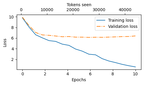

从结果来看，模型最初生成的单词串难以理解，但随着训练的进行，它能够生成语法基本正确的句子。然而，训练集和验证集的损失值表明模型出现了过拟合：在训练后期生成的文本段落与训练集内容完全一致，说明模型只是简单地记住了训练数据。后续将介绍一些解码策略来缓解这种记忆现象。需要注意的是，过拟合的原因在于使用了非常小的训练集并进行了多次迭代：

本次大语言模型（LLM）训练主要是为了教育目的，旨在观察模型是否能学会生成连贯文本.
为了避免在昂贵硬件上花费数周或数月时间训练模型，后续会加载预训练权重

5.3 Decoding strategies to control randomness

以下是重新组织并精简后的内容：

在本节中，我们将介绍文本生成策略（也称为解码策略）以生成更具原创性的文本。首先，简要回顾前一章的 generate_text_simple 函数，该函数之前用于 generate_and_print_sample 中。接着，介绍两种改进该函数的技术：
1. 温度调节（temperature scaling）
2. top-k 采样（top-k sampling）.
我们首先将模型从 GPU 转移回 CPU，因为对于相对较小的模型来说，推理（inference）不需要 GPU。此外，在训练结束后，我们将模型设置为评估模式（evaluation mode），以关闭随机组件，例如 dropout。接下来，我们将 GPTModel 实例（模型）插入到generate_text_simple函数中，该函数使用 LLM 一次生成一个token：
```
model.to("cpu")
model.eval()

tokenizer = tiktoken.get_encoding("gpt2")

token_ids = generate_text_simple(
    model=model,
    idx=text_to_token_ids("Every effort moves you", tokenizer),
    max_new_tokens=25,
    context_size=GPT_CONFIG_124M["context_length"]
)

print("Output text:\n", token_ids_to_text(token_ids, tokenizer))

"""输出"""
Output text:
 Every effort moves you?"

"Yes--quite insensible to the irony. She wanted him vindicated--and by me!"
```
我们已知，在每个生成步骤中选择生成的标记，对应于词汇表中所有标记中的最大概率分数。这意味着即使我们在同一台计算机上多次运行上面的 generate_text_simple 函数，大语言模型（LLM）也将始终生成相同的输出。 因此，后续两个小节介绍的两个概念，用于控制生成文本的随机性和多样性：温度调节（temperature scaling）和 top-k 采样（top-k sampling）。

5.3.1 Temperature scaling

此前，在generate_text_simple函数中，我们总是使用torch.argmax采样概率最高的token作为下一个token，这种方式也被称为greedy decoding。为了生成更多样化的文本，我们可以将argmax替换为一个从概率分布中采样的函数torch.multinomial(probs, num_samples=1)（这里的概率分布是指LLM在每一步token生成时为词汇表中每个条目生成的概率分数）。

为了通过具体示例说明概率采样，我们简要讨论下一个标记生成过程，并使用一个非常小的词汇表进行说明
```
vocab = { 
    "closer": 0,
    "every": 1, 
    "effort": 2, 
    "forward": 3,
    "inches": 4,
    "moves": 5, 
    "pizza": 6,
    "toward": 7,
    "you": 8,
} 

inverse_vocab = {v: k for k, v in vocab.items()}

# 假设 LLM 被赋予起始上下文“every effort moves you”，并生成以下下一个令牌逻辑
next_token_logits = torch.tensor(
    [4.51, 0.89, -1.90, 6.75, 1.63, -1.62, -1.89, 6.28, 1.79]
)

probas = torch.softmax(next_token_logits, dim=0)
next_token_id = torch.argmax(probas).item()

# The next generated token is then as follows:
print(inverse_vocab[next_token_id])

"""输出"""
forward
```
由于最大的 logit 值以及相应的最大的 softmax 概率得分位于第四个位置（索引位置 3，因为 Python 使用 0 索引），因此生成的单词是“forward”。

为了实现概率采样过程，我们现在可以替换argmax 与 PyTorch 中的multinomial函数：
```
torch.manual_seed(123)
next_token_id = torch.multinomial(probas, num_samples=1).item()
print(inverse_vocab[next_token_id])

"""输出"""
toward
```
我们使用torch.multinomial(probas, num_samples=1)从softmax分布中采样确定最可能的token，而非直接使用torch.argmax。为便于说明，观察使用原始softmax概率对下一个token进行1,000次采样的结果
```
def print_sampled_tokens(probas):
    torch.manual_seed(123) # Manual seed for reproducibility
    sample = [torch.multinomial(probas, num_samples=1).item() for i in range(1_000)]
    sampled_ids = torch.bincount(torch.tensor(sample))
    for i, freq in enumerate(sampled_ids):
        print(f"{inverse_vocab[i]}\t x \t {freq}")

print_sampled_tokens(probas)

"""输出"""
closer	 x 	 71
every	 x 	 2
effort	 x 	 0
forward	 x 	 544
inches	 x 	 2
moves	 x 	 1
pizza	 x 	 0
toward	 x 	 376
you	 x 	 4
```
从输出中可以看出，单词“forward”被采样的次数最多（1000次中有544次），但是其他token如closer,toward偶尔也会被采样。这意味着，如果我们在generate_and_print_sample函数中用multinomial函数替换argmax函数，LLM有时会生成诸如“every effort moves you toward”“every effort moves you inches”和“every effort moves you closer”的文本，而不仅仅是“every effort moves you forward”。

我们可以通过一种称为“temperature scaling”的概念进一步控制分布和选择过程，其中“temperature scaling”只是一个花哨的描述，指的是将logits除以一个大于0的数：

def softmax_with_temperature(logits, temperature):
    scaled_logits = logits / temperature
    return torch.softmax(scaled_logits, dim=0)

# Temperature values
temperatures = [1, 0.1, 5]  # Original, higher confidence, and lower confidence

# Calculate scaled probabilities
scaled_probas = [softmax_with_temperature(next_token_logits, T) for T in temperatures]

# Plotting
x = torch.arange(len(vocab))
bar_width = 0.15

fig, ax = plt.subplots(figsize=(5, 3))
for i, T in enumerate(temperatures):
    rects = ax.bar(x + i * bar_width, scaled_probas[i], bar_width, label=f'Temperature = {T}')

ax.set_ylabel('Probability')
ax.set_xticks(x)
ax.set_xticklabels(vocab.keys(), rotation=90)
ax.legend()

plt.tight_layout()
plt.savefig("temperature-plot.pdf")
plt.show()

温度值大于1会导致token概率分布更加均匀，而温度值小于1则会导致分布更加集中（更尖锐或更突出）我们通过绘制原始概率与不同温度值缩放后的概率来直观说明这一点：

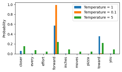
我们可以看到

温度值为1时等同于无缩放，token选择概率与原始softmax一致；

print_sampled_tokens(scaled_probas[0]) # temperature=1

"""输出"""
closer	 x 	 71
every	 x 	 2
effort	 x 	 0
forward	 x 	 544
inches	 x 	 2
moves	 x 	 1
pizza	 x 	 0
toward	 x 	 376
you	     x 	 4

温度值小于1（如0.1）时分布更尖锐，接近torch.argmax的效果，几乎总是选择最可能的token；

print_sampled_tokens(scaled_probas[1]) # temperature=0.1

"""输出"""
closer	 x 	 0
every	 x 	 0
effort	 x 	 0
forward	 x 	 992
inches	 x 	 0
moves	 x 	 0
pizza	 x 	 0
toward	 x 	 8

温度值大于1（如5）时分布更均匀，增加文本多样性但可能导致无意义内容，如

every effort moves you pizza（pizza出现了43次，概率为4.3%）

print_sampled_tokens(scaled_probas[2]) # temperature=5

"""输出"""
closer	 x 	 153
every	 x 	 68
effort	 x 	 55
forward	 x 	 223
inches	 x 	 102
moves	 x 	 50
pizza	 x 	 43
toward	 x 	 218
you	     x 	 88

5.3.2 Top-k sampling

在上一节中，我们通过结合温度缩放的概率采样方法增加了输出多样性，较高温度值使token分布更均匀，减少重复选择最可能token的情况，从而探索更具创造性的路径，但这种方法有时会导致语法错误或完全无意义的输出（如“every effort moves you pizza”）。

为了能够使用较高的温度值来增加输出多样性并减少无意义句子的概率，我们可以将采样的token限制在top-k最可能的token中：

使用 k=3 的 top-k 采样，我们关注与最高 logits 相关的 3 个标记，并在应用 softmax 函数之前屏蔽掉所有其他具有负无穷大 (-inf) 的标记。这会导致概率分布的概率值为 0 分配给所有非前 k 个标记。

在代码中实现上图中概述的 top-k 过程

首先选择具有最大 logit 值的标记：

top_k = 3
top_logits, top_pos = torch.topk(next_token_logits, top_k)

print("Top logits:", top_logits)
print("Top positions:", top_pos)

"""输出"""
Top logits: tensor([6.7500, 6.2800, 4.5100])
Top positions: tensor([3, 7, 0])

随后，我们应用 PyTorch 的 where 函数将低于 top-3 选择中最低 logit 值的标记的 logit 值设置为负无穷大 (-inf)

new_logits = torch.where(
    condition=next_token_logits < top_logits[-1],
    input=torch.tensor(float("-inf")), 
    other=next_token_logits
)
# 或者
# new_logits = torch.full_like( # 创建一个包含-inf值的张量  
#    next_token_logits, -torch.inf  
# )   
# new_logits[top_pos] = next_token_logits[top_pos] # 将top k值复制到-inf张量中  

print(new_logits)


"""输出"""
tensor([4.5100, -inf, -inf, 6.7500, -inf, -inf, -inf, 6.2800, -inf])

最后，让我们应用 softmax 函数将它们转换为下一个标记的概率：

topk_probas = torch.softmax(new_logits, dim=0)
print(topk_probas)

"""输出"""
tensor([0.0615, 0.00, 0.00, 0.5775, 0.00, 0.00, 0.00, 0.3610, 0.00])

5.3.3 Modifying the text generation function

前两小节介绍了温度采样（temperature sampling）和top-k采样（top-k sampling），我们将利用这两个概念修改之前用于通过LLM生成文本的generate_simple函数，创建一个新的generate函数。

def generate(model, idx, max_new_tokens, context_size, temperature=0.0, top_k=None, eos_id=None):

    # For-loop is the same as before: Get logits, and only focus on last time step
    for _ in range(max_new_tokens):
        idx_cond = idx[:, -context_size:]
        with torch.no_grad():
            logits = model(idx_cond)
        logits = logits[:, -1, :]

        # New: Filter logits with top_k sampling
        if top_k is not None:
            # Keep only top_k values
            top_logits, _ = torch.topk(logits, top_k)
            min_val = top_logits[:, -1]
            logits = torch.where(logits < min_val, torch.tensor(float("-inf")).to(logits.device), logits)

        # New: Apply temperature scaling
        if temperature > 0.0:
            logits = logits / temperature

            # Apply softmax to get probabilities
            probs = torch.softmax(logits, dim=-1)  # (batch_size, context_len)

            # Sample from the distribution
            idx_next = torch.multinomial(probs, num_samples=1)  # (batch_size, 1)

        # Otherwise same as before: get idx of the vocab entry with the highest logits value
        else:
            idx_next = torch.argmax(logits, dim=-1, keepdim=True)  # (batch_size, 1)

        if idx_next == eos_id:  # Stop generating early if end-of-sequence token is encountered and eos_id is specified
            break

        # Same as before: append sampled index to the running sequence
        idx = torch.cat((idx, idx_next), dim=1)  # (batch_size, num_tokens+1)

    return idx

更改完成后，看看这个新生成函数的实际效果

torch.manual_seed(123)

token_ids = generate(
    model=model,
    idx=text_to_token_ids("Every effort moves you", tokenizer),
    max_new_tokens=15,
    context_size=GPT_CONFIG_124M["context_length"],
    top_k=25,
    temperature=1.4
)

print("Output text:\n", token_ids_to_text(token_ids, tokenizer))

"""输出"""
Output text:
 Every effort moves you know began to my surprise, poor StI was such a good; and

下面的是我们先前生成的output

 Every effort moves you?"

"Yes--quite insensible to the irony. She wanted him vindicated--and by me!"

可以对比一下，已经有很大的不同了。

5.4 Loading and saving model weights in PyTorch

训练LLM的计算成本很高，因此能够保存和加载LLM的权重至关重要。

在PyTorch中，推荐的方式是通过将torch.save函数应用于.state_dict()方法来保存模型权重，即所谓的state_dict：

torch.save(model.state_dict(),"model.pth")

我们可以将模型权重加载到新的 GPTModel 模型实例中

model = GPTModel(GPT_CONFIG_124M)
device = torch.device("cuda" if torch.cuda.is_available() else "cpu")
model.load_state_dict(torch.load("model.pth", map_location=device, weights_only=True))
model.eval();

自适应优化器（如 AdamW）为每个模型权重存储额外的参数。AdamW 使用历史数据动态调整每个模型参数的学习率。如果没有这些参数，优化器会重置，模型可能会学习效果不佳，甚至无法正确收敛，这意味着模型将失去生成连贯文本的能力。使用 torch.save，我们可以保存模型和优化器的 state_dict 内容，如下所示
```
torch.save({
    "model_state_dict": model.state_dict(),
    "optimizer_state_dict": optimizer.state_dict(),
    }, 
    "model_and_optimizer.pth"
)
```
然后，我们可以通过以下方式恢复模型和优化器状态：首先通过 torch.load 加载保存的数据，然后使用 load_state_dict 方法：
```
checkpoint = torch.load("model_and_optimizer.pth", weights_only=True)

model = GPTModel(GPT_CONFIG_124M)
model.load_state_dict(checkpoint["model_state_dict"])

optimizer = torch.optim.AdamW(model.parameters(), lr=0.0005, weight_decay=0.1)
optimizer.load_state_dict(checkpoint["optimizer_state_dict"])
model.train();
```

5.5 Loading pretrained weights from OpenAI

此前用于教学目的，我们仅使用一本非常短的故事书训练了一个小型GPT-2模型，幸运的是，我们无需花费数万到数十万美元在大型预训练语料库上预训练模型，而是可以加载OpenAI提供的预训练权重(OpenAI 公开分享了他们的 GPT-2 模型的权重)。由于OpenAI使用了TensorFlow，我们需要安装并使用TensorFlow来加载权重；

这里作者给了个代码 gpt_download.py 文件，从本章的在线仓库下载

在线仓库地址

https://github.com/rasbt/LLMs-fromscratch

# Copyright (c) Sebastian Raschka under Apache License 2.0 (see LICENSE.txt).
# Source for "Build a Large Language Model From Scratch"
#   - https://www.manning.com/books/build-a-large-language-model-from-scratch
# Code: https://github.com/rasbt/LLMs-from-scratch


import os
import urllib.request

# import requests
import json
import numpy as np
import tensorflow as tf
from tqdm import tqdm


def download_and_load_gpt2(model_size, models_dir):
    # Validate model size
    allowed_sizes = ("124M", "355M", "774M", "1558M")
    if model_size not in allowed_sizes:
        raise ValueError(f"Model size not in {allowed_sizes}")

    # Define paths
    model_dir = os.path.join(models_dir, model_size)
    base_url = "https://openaipublic.blob.core.windows.net/gpt-2/models"
    filenames = [
        "checkpoint", "encoder.json", "hparams.json",
        "model.ckpt.data-00000-of-00001", "model.ckpt.index",
        "model.ckpt.meta", "vocab.bpe"
    ]

    # Download files
    os.makedirs(model_dir, exist_ok=True)
    for filename in filenames:
        file_url = os.path.join(base_url, model_size, filename)
        file_path = os.path.join(model_dir, filename)
        download_file(file_url, file_path)

    # Load settings and params
    tf_ckpt_path = tf.train.latest_checkpoint(model_dir)
    settings = json.load(open(os.path.join(model_dir, "hparams.json")))
    params = load_gpt2_params_from_tf_ckpt(tf_ckpt_path, settings)

    return settings, params


def download_file(url, destination):
    # Send a GET request to download the file

    try:
        with urllib.request.urlopen(url) as response:
            # Get the total file size from headers, defaulting to 0 if not present
            file_size = int(response.headers.get("Content-Length", 0))

            # Check if file exists and has the same size
            if os.path.exists(destination):
                file_size_local = os.path.getsize(destination)
                if file_size == file_size_local:
                    print(f"File already exists and is up-to-date: {destination}")
                    return

            # Define the block size for reading the file
            block_size = 1024  # 1 Kilobyte

            # Initialize the progress bar with total file size
            progress_bar_description = os.path.basename(url)  # Extract filename from URL
            with tqdm(total=file_size, unit="iB", unit_scale=True, desc=progress_bar_description) as progress_bar:
                # Open the destination file in binary write mode
                with open(destination, "wb") as file:
                    # Read the file in chunks and write to destination
                    while True:
                        chunk = response.read(block_size)
                        if not chunk:
                            break
                        file.write(chunk)
                        progress_bar.update(len(chunk))  # Update progress bar
    except urllib.error.HTTPError:
        s = (
            f"The specified URL ({url}) is incorrect, the internet connection cannot be established,"
            "\nor the requested file is temporarily unavailable.\nPlease visit the following website"
            " for help: https://github.com/rasbt/LLMs-from-scratch/discussions/273")
        print(s)


# Alternative way using `requests`
"""
def download_file(url, destination):
    # Send a GET request to download the file in streaming mode
    response = requests.get(url, stream=True)

    # Get the total file size from headers, defaulting to 0 if not present
    file_size = int(response.headers.get("content-length", 0))

    # Check if file exists and has the same size
    if os.path.exists(destination):
        file_size_local = os.path.getsize(destination)
        if file_size == file_size_local:
            print(f"File already exists and is up-to-date: {destination}")
            return

    # Define the block size for reading the file
    block_size = 1024  # 1 Kilobyte

    # Initialize the progress bar with total file size
    progress_bar_description = url.split("/")[-1]  # Extract filename from URL
    with tqdm(total=file_size, unit="iB", unit_scale=True, desc=progress_bar_description) as progress_bar:
        # Open the destination file in binary write mode
        with open(destination, "wb") as file:
            # Iterate over the file data in chunks
            for chunk in response.iter_content(block_size):
                progress_bar.update(len(chunk))  # Update progress bar
                file.write(chunk)  # Write the chunk to the file
"""


def load_gpt2_params_from_tf_ckpt(ckpt_path, settings):
    # Initialize parameters dictionary with empty blocks for each layer
    params = {"blocks": [{} for _ in range(settings["n_layer"])]}

    # Iterate over each variable in the checkpoint
    for name, _ in tf.train.list_variables(ckpt_path):
        # Load the variable and remove singleton dimensions
        variable_array = np.squeeze(tf.train.load_variable(ckpt_path, name))

        # Process the variable name to extract relevant parts
        variable_name_parts = name.split("/")[1:]  # Skip the 'model/' prefix

        # Identify the target dictionary for the variable
        target_dict = params
        if variable_name_parts[0].startswith("h"):
            layer_number = int(variable_name_parts[0][1:])
            target_dict = params["blocks"][layer_number]

        # Recursively access or create nested dictionaries
        for key in variable_name_parts[1:-1]:
            target_dict = target_dict.setdefault(key, {})

        # Assign the variable array to the last key
        last_key = variable_name_parts[-1]
        target_dict[last_key] = variable_array

    return params

下载123m参数的模型参数

注意更改下自己的models_dir

from gpt_download import download_and_load_gpt2
settings, params = download_and_load_gpt2(model_size="124M",models_dir="E:\\LLM\\gpt2\\")

"""输出"""
checkpoint: 100%|███████████████████████████| 77.0/77.0 [ 26.5kiB/s]
encoder.json: 100%|█████████████████████████| 1.04M/1.04M [810 kiB/s]
hprams.json: 100%|██████████████████████████| 90.0/90.0 [78.3kiB/s]
model.ckpt.data-00000-of-00001: 100%|███████| 498M/498M [7.16MiB/s]
model.ckpt.index: 100%|█████████████████████| 5.21k/5.21k [3.24kiB/s]
model.ckpt.meta: 100%|██████████████████████| 471k/471k [2.46MiB/s]
vocab.bpe: 100%|████████████████████████████| 456k/456k [20.5kiB/s]

setting字典存储LLM架构设置，类似于我们手动定义的GPT_CONFIG_124M 设置

print("Settings:", settings)

"""输出"""
Settings: {'n_vocab': 50257, 'n_ctx': 1024, 'n_embd': 768, 'n_head': 12, 'n_layer': 12}

params 字典包含实际的权重张量（这里只打印了键）

print("Parameter dictionary keys:", params.keys())

"""输出"""
Parameter dictionary keys: dict_keys(['blocks', 'b', 'g', 'wpe', 'wte'])

blocks: 表示 GPT 模型中的 Transformer 块（Transformer blocks）。每个块包含自注意力机制（self-attention）和前馈神经网络（feed-forward network）等核心组件。这些块堆叠在一起，构成了 GPT 模型的多层结构
b 通常表示模型中的偏置项（bias）
g 通常与层归一化（Layer Normalization）相关，表示归一化层中的缩放参数（scale parameter）。在 Transformer 模型中，层归一化用于稳定训练过程
wpe 表示位置编码的权重矩阵（Positional Encoding weights）。由于 Transformer 模型本身不包含序列顺序信息，位置编码用于为输入序列中的每个位置添加唯一的位置信息
wte 表示词嵌入的权重矩阵（Word Token Embedding weights）。它将输入的单词或标记（token）映射到高维向量空间，捕捉词汇的语义信息

我们通过相应字典键选择单个张量来检查这些权重张量，例如，嵌入层权重：

print(params["wte"])
print("Token embedding weight tensor dimensions:", params["wte"].shape)

"""输出"""
[[-0.11010301 -0.03926672  0.03310751 ... -0.1363697   0.01506208
   0.04531523]
 [ 0.04034033 -0.04861503  0.04624869 ...  0.08605453  0.00253983
   0.04318958]
 [-0.12746179  0.04793796  0.18410145 ...  0.08991534 -0.12972379
  -0.08785918]
 ...
 [-0.04453601 -0.05483596  0.01225674 ...  0.10435229  0.09783269
  -0.06952604]
 [ 0.1860082   0.01665728  0.04611587 ... -0.09625227  0.07847701
  -0.02245961]
 [ 0.05135201 -0.02768905  0.0499369  ...  0.00704835  0.15519823
   0.12067825]]
Token embedding weight tensor dimensions: (50257, 768)

此外，“355M”“774M”和“1558M”也是支持的model_size参数。这些不同大小模型之间的差异总结如下图所示：

GPT-2 LLMs 有多种不同的模型大小，参数范围从 1.24 亿到 15.58 亿个参数不等。核心架构是相同的，唯一的区别是嵌入大小和单个组件（如注意力头和变压器块）重复的次数。

在将124M GPT-2模型权重加载到Python后，我们初始化了一个新的GPTModel实例，并启用了qkv_bias以正确加载权重，同时使用了原始GPT-2模型的1024个token的上下文长度。

我们先创建一个字典，列出不同GPT模型大小之间如上图所示的差异

# Define model configurations in a dictionary for compactness
model_configs = {
    "gpt2-small (124M)": {"emb_dim": 768, "n_layers": 12, "n_heads": 12},
    "gpt2-medium (355M)": {"emb_dim": 1024, "n_layers": 24, "n_heads": 16},
    "gpt2-large (774M)": {"emb_dim": 1280, "n_layers": 36, "n_heads": 20},
    "gpt2-xl (1558M)": {"emb_dim": 1600, "n_layers": 48, "n_heads": 25},
}

加载最小的模型 gpt2-small(124m)

# Copy the base configuration and update with specific model settings
model_name = "gpt2-small (124M)"  # Example model name
NEW_CONFIG = GPT_CONFIG_124M.copy()
NEW_CONFIG.update(model_configs[model_name])

我们这里之前使用256个token长度，但是OpenAI原始GPT-2模型是用1024个令牌长度训练的,此外OpenAI 在多头注意力模块的线性层中使用偏差向量来实现查询、键和值矩阵计算。偏差向量在 LLMs 中不再常用，因为它们不会提高建模性能，因此没有必要。但是，由于我们正在使用预训练的权重，因此我们需要匹配设置以确保一致性并启用这些偏差向量：

NEW_CONFIG.update({"context_length": 1024, "qkv_bias": True})

gpt = GPTModel(NEW_CONFIG)
gpt.eval();

接下来的任务是将OpenAI的权重分配到我们GPTModel实例中对应的权重张量中。

def assign(left, right):
    if left.shape != right.shape:
        raise ValueError(f"Shape mismatch. Left: {left.shape}, Right: {right.shape}")
    return torch.nn.Parameter(torch.tensor(right))

定义一个 load_weights_into_gpt 函数，它将 params 字典中的权重加载到 GPTModel 实例 gpt 中：

import numpy as np

def load_weights_into_gpt(gpt, params):
    gpt.pos_emb.weight = assign(gpt.pos_emb.weight, params['wpe'])
    gpt.tok_emb.weight = assign(gpt.tok_emb.weight, params['wte'])
    
    for b in range(len(params["blocks"])):
        q_w, k_w, v_w = np.split(
            (params["blocks"][b]["attn"]["c_attn"])["w"], 3, axis=-1)
        gpt.trf_blocks[b].att.W_query.weight = assign(
            gpt.trf_blocks[b].att.W_query.weight, q_w.T)
        gpt.trf_blocks[b].att.W_key.weight = assign(
            gpt.trf_blocks[b].att.W_key.weight, k_w.T)
        gpt.trf_blocks[b].att.W_value.weight = assign(
            gpt.trf_blocks[b].att.W_value.weight, v_w.T)

        q_b, k_b, v_b = np.split(
            (params["blocks"][b]["attn"]["c_attn"])["b"], 3, axis=-1)
        gpt.trf_blocks[b].att.W_query.bias = assign(
            gpt.trf_blocks[b].att.W_query.bias, q_b)
        gpt.trf_blocks[b].att.W_key.bias = assign(
            gpt.trf_blocks[b].att.W_key.bias, k_b)
        gpt.trf_blocks[b].att.W_value.bias = assign(
            gpt.trf_blocks[b].att.W_value.bias, v_b)

        gpt.trf_blocks[b].att.out_proj.weight = assign(
            gpt.trf_blocks[b].att.out_proj.weight, 
            params["blocks"][b]["attn"]["c_proj"]["w"].T)
        gpt.trf_blocks[b].att.out_proj.bias = assign(
            gpt.trf_blocks[b].att.out_proj.bias, 
            params["blocks"][b]["attn"]["c_proj"]["b"])

        gpt.trf_blocks[b].ff.layers[0].weight = assign(
            gpt.trf_blocks[b].ff.layers[0].weight, 
            params["blocks"][b]["mlp"]["c_fc"]["w"].T)
        gpt.trf_blocks[b].ff.layers[0].bias = assign(
            gpt.trf_blocks[b].ff.layers[0].bias, 
            params["blocks"][b]["mlp"]["c_fc"]["b"])
        gpt.trf_blocks[b].ff.layers[2].weight = assign(
            gpt.trf_blocks[b].ff.layers[2].weight, 
            params["blocks"][b]["mlp"]["c_proj"]["w"].T)
        gpt.trf_blocks[b].ff.layers[2].bias = assign(
            gpt.trf_blocks[b].ff.layers[2].bias, 
            params["blocks"][b]["mlp"]["c_proj"]["b"])

        gpt.trf_blocks[b].norm1.scale = assign(
            gpt.trf_blocks[b].norm1.scale, 
            params["blocks"][b]["ln_1"]["g"])
        gpt.trf_blocks[b].norm1.shift = assign(
            gpt.trf_blocks[b].norm1.shift, 
            params["blocks"][b]["ln_1"]["b"])
        gpt.trf_blocks[b].norm2.scale = assign(
            gpt.trf_blocks[b].norm2.scale, 
            params["blocks"][b]["ln_2"]["g"])
        gpt.trf_blocks[b].norm2.shift = assign(
            gpt.trf_blocks[b].norm2.shift, 
            params["blocks"][b]["ln_2"]["b"])

    gpt.final_norm.scale = assign(gpt.final_norm.scale, params["g"])
    gpt.final_norm.shift = assign(gpt.final_norm.shift, params["b"])
    gpt.out_head.weight = assign(gpt.out_head.weight, params["wte"])
    
    
load_weights_into_gpt(gpt, params)
gpt.to(device);

在load_weights_into_gpt函数中，我们仔细地将OpenAI实现中的权重与我们的GPTModel实现进行匹配。以具体示例为例，OpenAI将第一个Transformer块的输出投影层的权重张量存储为params["blocks"][0]["attn"]["c_proj"]["w"]。在我们的实现中，该权重张量对应于gpt.trf_blocks[b].att.out_proj.weight，其中gpt是GPTModel的一个实例。

由于 OpenAI 使用的命名约定与我们的命名约定略有不同，因此开发 load_weights_into_gpt 函数需要进行大量猜测。但是，如果我们尝试匹配两个具有不同维度的张量，则分配函数会提醒我们。此外，如果我们在此函数中犯了错误，我们会注意到这一点，因为生成的 GPT 模型将无法生成连贯的文本。

如果模型加载正确，我们可以使用之前的generate函数生成新文本

torch.manual_seed(123)

token_ids = generate(
    model=gpt,
    idx=text_to_token_ids("Every effort moves you", tokenizer).to(device),
    max_new_tokens=25,
    context_size=NEW_CONFIG["context_length"],
    top_k=50,
    temperature=1.5
)

print("Output text:\n", token_ids_to_text(token_ids, tokenizer))


"""输出"""
Output text:
 Every effort moves you as far as the hand can go until the end of your turn unless something happens

This would remove you from a battle

5.6 Summary

When LLMs generate text, they output one token at a time.
By default, the next token is generated by converting the model outputs into probability scores and selecting the token from the vocabulary that corresponds to the highest probability score, which is known as “greedy decoding.”
Using probabilistic sampling and temperature scaling, we can influence the diversity and coherence of the generated text.
Training and validation set losses can be used to gauge the quality of text generated by LLM during training.
Pretraining an LLM involves changing its weights to minimize the training loss.
The training loop for LLMs itself is a standard procedure in deep learning, using a conventional cross entropy loss and AdamW optimizer.
Pretraining an LLM on a large text corpus is time- and resource-intensive so we can load openly available weights from OpenAI as an alternative to pretraining the model on a large dataset ourselves.
1. 文本生成过程：
  - LLM生成文本时，每次输出一个token。
  - 默认情况下，通过将模型输出转换为概率分数并选择概率最高的token（称为“贪婪解码”）来生成下一个token。
2. 多样性与连贯性控制：
  - 使用概率采样（probabilistic sampling）和温度缩放（temperature scaling）可以影响生成文本的多样性和连贯性。
3. 训练与验证损失：
  - 训练和验证集的损失可用于评估LLM在训练期间生成的文本质量。
4. 预训练过程：
  - 预训练LLM涉及调整其权重以最小化训练损失。
  - LLM的训练循环是深度学习的标准过程，使用传统的交叉熵损失（cross entropy loss）和AdamW优化器。
5. 预训练的挑战与替代方案：
  - 在大型文本语料库上预训练LLM耗时且资源密集。
  - 作为替代方案，可以加载OpenAI公开的权重，而无需自己在大型数据集上进行预训练。