


原文链接:https://pytorch.org/tutorials/beginner/deep_learning_60min_blitz.html
这个教程的目标是:
- 对PyTorch的张量和神经网络有大致的了解
- 训练一个小的图片分类的神经网络。
本教程假设你对numpy有一个基础的了解
注意:确保你已经安装了torch和torchvision模块
目录
什么是PyTorch?
它是一个基于Python的科学计算软件包。主要针对两类受众:
- 使用GPU运算来取代Numpy
- 提供最大灵活性和速度的深度学习研究平台
入门
张量(Tensors)
张量和Numpy的ndarray类似。不同的是张量可以在GPU上运行以加速运算。
使用张量构造一个未初始化的5*3的矩阵:
import torch
x=torch.empty(5,3)
print(x)
输出:
tensor([[ 5.3209e-09,  3.0918e-41,  5.3422e-09],
        [ 3.0918e-41,  5.6460e-09,  3.0918e-41],
        [ 5.8182e-09,  3.0918e-41,  2.1418e-39],
        [ 1.6714e-38,  1.7853e-37,  0.0000e+00],
        [ 3.8169e-40,  2.7142e-24,  1.3744e+11]])
构造一个随机数据的矩阵:
x=torch.rand(5,3)
print(x)
输出:
tensor([[ 0.8983,  0.1658,  0.5158],
        [ 0.8509,  0.9362,  0.5348],
        [ 0.5108,  0.8170,  0.6949],
        [ 0.1138,  0.3153,  0.4799],
        [ 0.2695,  0.4061,  0.9428]])
构造一个dtype为long的全0矩阵:
x=torch.zeros(5,3,dtype=torch.long)
print(x)
输出:
tensor([[ 0,  0,  0],
        [ 0,  0,  0],
        [ 0,  0,  0],
        [ 0,  0,  0],
        [ 0,  0,  0]])
直接通过数据来构造张量:
x=torch.tensor([5.5,3])
print(x)
输出:
tensor([ 5.5000, 3.0000])或基于已有张量来创建张量。除非用户提供新的值,否则这些方法将重用输入张量的属性,例如dtype。
x=x.new_ones(5,3,dtype=torch.double) #方法new_* 的参数是张量的大小
print(x)
x=torch.randn_like(x,dtype=torch.float)#重新定义了dtype
print(x)#保留了原来张量的大小
输出:
tensor([[ 1.,  1.,  1.],
        [ 1.,  1.,  1.],
        [ 1.,  1.,  1.],
        [ 1.,  1.,  1.],
        [ 1.,  1.,  1.]], dtype=torch.float64)
tensor([[ 0.6536, -0.0688, -0.4559],
        [ 0.4712,  1.0297,  0.5794],
        [ 0.7719,  0.5049, -2.1100],
        [-1.0550, -1.3705, -0.7813],
        [-1.2648,  0.5148,  0.2817]])
获取张量的形状:
print(x.size())输出:
(5, 3)注意:
torch.size实际上是一个tuple(元组),所以它支持所有元组的运算。
运算(Operations)
运算有很多种语法。接下来的例子我们看下加法运算。
加法:语法1
y=torch.rand(5,3)
print(x+y)
输出(接下来的语法,输出都相同):
tensor([[ 1.3995, -0.4390, -0.2863],
        [ 0.6528,  1.3047, -0.5661],
        [ 1.4773,  0.8449, -1.7209],
        [-0.3371,  1.0313, -0.1698],
        [-0.6412, -0.7284, -0.9708]])
加法:语法2
print(torch.add(x,y))加法:提供一个输出张量作为参数
result=torch.empty(5,3)
torch.add(x,y,out=result)
print(result)
加法:in-place(不再有输出变量。运算结果直接赋值给调用者)
y.add_(x)
print(y)
注意:
任何运算方法名后面加“_”都代表in-place。例如:x.copy_(y),x.t_(),都会改变x。
你可以使用标准的Numpy风格的索引操作。
print(x[:,1])输出:
tensor([ 1.0198, -2.2140, -0.3281, -1.1494, -0.9980])调整大小:如果你想要改变张量的形状,可以使用torch.view:
x=torch.randn(4,4)
y=x.view(16)
z=x.view(-1,8)#-1代表通过其它维度推断获取
print(x.size(),y.size(),z.size())
输出:
((4, 4), (16,), (2, 8))如果张量只有一个元素,使用.item()可以获取它的Python数字的值,
x=torch.randn(1)
print(x)
print(x.item())
输出:
0.931114792824Numpy Bridge(与Numpy的转换)
Torch的张量和Numpy的数组将共享底层的内存位置,更改一个另一个也会改变。
Torch的张量到Numpy数组的转换
a=torch.ones(5)
print(a)

b=a.numpy()
print(b)
输出:
tensor([ 1.,  1.,  1.,  1.,  1.])
[1. 1. 1. 1. 1.]
torch的张量改变时numpy数组也随着改变
a.add_(1)
print(a)
print(b)
输出:
tensor([ 2.,  2.,  2.,  2.,  2.])
[2. 2. 2. 2. 2.]
Numpy数组转换为Torch张量
改变Numpy数组时Torch张量也跟着改变
import numpy as np
a=np.ones(5)
b=torch.from_numpy(a)
np.add(a,1,out =a)
print(a)
print(b)
输出:
[2. 2. 2. 2. 2.]
tensor([ 2.,  2.,  2.,  2.,  2.], dtype=torch.float64)
在CPU上所有的张量(CharTensor除外)均支持与Numpy的转换。
Autograd:自动微分
autograd package是PyTorch神经网络的核心。我们先简单看一下,然后开始训练第一个神经网络。
autograd package为张量的所有operations(操作或运算)提供了自动微分。它是一个 define-by-run框架,意思是说你的反向传播(backpropagation)是由 如何运行代码 定义的,并且每一个迭代可以是不同的。
用例子和一些简单的术语来看下:
Tensor(张量)
torch.Tensor是包的核心类。如果你设置它的.requires_grad属性 为 True,它的所有操作都会被跟踪记录。完成计算后可以调用.backward()方法,并自动计算所有的梯度。这个张量的梯度将会被累积到.grad属性。
你可以调用.detach()方法来阻止张量对所有操作的跟踪记录。
阻止跟踪历史的另一种方法是你在代码块外包裹语句 with torch.no_grad(): ,这种方法在模型中训练参数设置了requires_grad=True时依然有效。
实现自动微分的另一个重要的类是Function.(这里function可理解为一个运算。比如加法运算)
Tensor 和 Function相互关联建立了一个非循环图,它记录了完整的计算历史。每一个张量有一个.grad_fn属性,这个属性与创建张量(除了用户自己创建的张量,它们的.grad_fn是None)的Function关联。
如果你想要计算导数,你可以调用张量的.backward()方法。如果张量是一个标量(例如,它只有一个元素),你不需要指定backward()的参数,然而,如果张量有多个元素,你需要指定一个匹配张量大小的gradient参数。
import torch创建一个张量,并设置requires_grad=True来跟踪计算。
x=torch.ones(2,2,requires_grad=True)
print(x)
print(x.requires_grad)
输出:
tensor([[ 1.,  1.],
        [ 1.,  1.]])
True
对张量做一个运算,这里是+:
y=x+2
print(y)
输出:
tensor([[ 3.,  3.],
        [ 3.,  3.]])
y是被刚刚的运算(+)创建的,所以它有.grad_fn属性:
print(y.grad_fn)输出:
<AddBackward0 object at 0x7ff0cc6ca050>对y进行运算:
z=y*y*3
out=z.mean()
print(z,z.grad_fn)
print(out,out.grad_fn)
输出:
(tensor([[ 27.,  27.],
        [ 27.,  27.]]), <MulBackward0 object at 0x7f56c3a85050>)
(tensor(27.), <MeanBackward1 object at 0x7f56c3a85050>)
.requires_grad_(...)函数可以改变张量的requires_grad属性。如果该属性未给出,则默认为False。
a=torch.randn(2,2)
a=((a*3)/(a-1))
print(a.requires_grad)
a.requires_grad_(True)
print(a.requires_grad)
b=(a*a).sum()
print(b.grad_fn)
输出:
False
True
<SumBackward0 object at 0x7fcd902c2050>
梯度
有了自动微分,现在我们可以反向传播了。因为out只是一个简单的标量,out.backward()等价于out.backward(torch.tensor(1))
out.backward()打印出导数 d(out)/dx
print(x.grad)输出:
tensor([[ 4.5000,  4.5000],
        [ 4.5000,  4.5000]])
用下图来解释下为什么对out进行反向传播,x的梯度是4.5的矩阵吧:

你可以用自动微分做更多有趣的事。之前都是对标量进行backward(),不需要参数。下面看下是向量或矩阵时,gradient参数的值对梯度的影响:
x=torch.randn(3,requires_grad=True)
print(x)
y=x*2
while y.data.norm()<1000:
    y=y*2
#print(y)
gradients = torch.tensor([0.1,1.0,0.0001],dtype=torch.float)
y.backward(gradient=gradients)
print(x.grad)
输出:
tensor([ 0.9283, -0.7296,  0.1258])
tensor([ 102.4000, 1024.0000, 0.1024])如果你不想要跟踪历史并自动微分的时候,你可以在代码块外面包一层:with torch.no_grad():
print(x.requires_grad)
print((x**2).requires_grad)
with torch.no_grad():
    print((x**2).requires_grad)
输出:
True
True
False
神经网络
神经网络可以使用torch.nn package构造。
刚刚我们简单介绍了autograd,nn依赖于autograd来定义模型并区分它们。一个nn.Module包括你定义的网络层和一个forward(input)方法,这个方法返回output。
我们看下这个数字图片分类的网络的例子:
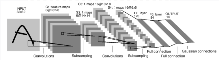
它是一个简单的前馈网络。它接受输入,并且每层的输入都是上一层的输出,最后给出输出。
一个典型的神经网络的训练过程如下:
- 定义具有学习参数(或权重)的神经网络
- 迭代输入数据集
- 根据神经网络对输入数据集进行运算
- 计算损失(输出与真实结果的距离。损失越小说明模型越准确。)
- 将梯度反向传播给神经网络的参数。
- 更新网络的权重(或参数)。通常使用一种简单的更新规则:权重=权重-学习率*梯度。
定义网络
来定义一个网络:
#encoding:utf-8
import torch
import torch.nn as nn
import torch.nn.functional as F

class Net(nn.Module):

    def __init__(self):
        super(Net,self).__init__()
        #定义2个卷积层
        self.conv1=nn.Conv2d(in_channels=1,out_channels=6,kernel_size=5)
        self.conv2=nn.Conv2d(in_channels=6,out_channels=16,kernel_size=5)
        #定义了3个线性层,即y=wx+b
        self.fc1=nn.Linear(in_features=16*5*5,out_features=120)
        self.fc2=nn.Linear(120,84)
        self.fc3=nn.Linear(84,10)

    def forward(self, x):
        #在第一层卷积网络和第二层之间增加了relu激活函数和池化层
        x=F.max_pool2d(input=F.relu(input=self.conv1(x)),kernel_size=(2,2))
        #如果池化层是方块形的可以用一个number指定
        x=F.max_pool2d(input=F.relu(input=self.conv2(x)),kernel_size=2)
        x=x.view(-1,self.num_flat_features(x))
        x=F.relu(input=self.fc1(x))
        x=F.relu(self.fc2(x))
        x=self.fc3(x)
        return x

    def num_flat_features(self,x):
        size=x.size()[1:]#切片0里面放的是当前训练batch的number,不是特征信息
        num_features=1
        for s in size:
            num_features*=s
        return num_features
net=Net()
print(net)
输出:
Net(
  (conv1): Conv2d(1, 6, kernel_size=(5, 5), stride=(1, 1))
  (conv2): Conv2d(6, 16, kernel_size=(5, 5), stride=(1, 1))
  (fc1): Linear(in_features=400, out_features=120, bias=True)
  (fc2): Linear(in_features=120, out_features=84, bias=True)
  (fc3): Linear(in_features=84, out_features=10, bias=True)
)你只需要定义forward方法,后向函数(自动计算微分的函数)就会自动定义,当然你需要设置autograd参数为True。在forward方法中你可以使用张量的任何运算。
模型的学习参数由net.parameters()返回。
params = list(net.parameters())
print(len(params))
print(params[0].size())  #conv1's .weight
输出:
10
(6, 1, 5, 5)这个网络适合32*32的数据集(1*32*32经过一个核心为5的卷积层,大小变为6*28*28;经过一个核心为2的池化层,大小变为6*14*14;再经过一个核心为5的卷积层,大小变为16*10*10;池化层,16*5*5,正好是下一个线性层的输入特征数),我们随机一个输入数据集,运行一下我们的模型吧:
input = torch.randn(1, 1, 32, 32)
out = net(input)
print(out)
输出:
tensor([[ 0.0567,  0.0185,  0.0279, -0.1414,  0.0109,  0.0566,  0.1015,
          0.0602,  0.0469,  0.0734]])
将梯度清0并使用随机梯度进行反向传播:
net.zero_grad()
out.backward(torch.randn(1,10))
注意
torch.nn 只支持对批量数据的处理,不支持单个样本。
例如,nn.Conv2d需要一个4维的张量作为输入:nSamples,nChannels,Height,Width.
如果你只有一个样本,你可以使用input.unsqueeze(0)来增加一个假的batch维。
在继续进行之前,我们回顾下刚学到的几个类。
torch.Tensor:一个支持自动微分(或梯度)操作(例如backward())的多维数组。
nn.Module: 神经网络模型,帮助我们封装参数,移植到GPU,导出,加载等的便捷方式。
nn.Parameter: 张量,当你给Module定义属性时,参数会自动生成。
autograd.Function:实现自动梯度运算的前向后向定义。每一个张量运算,产生至少一个Function节点,连接到创建张量的函数并对其历史进行编码。
在这个基础上,我们已经做了:
定义神经网络
处理输入和调用backward方法
还剩下:
计算损失
更新网络的权重
损失函数
一个损失函数包括两个输入(预测值和实际值),然后返回这两个值的距离。
在nn package里面有不同的损失函数。一个简单的损失函数是:nn.MSELoss,它返回的是均方差,即每一个分量相减的平方累计最后除分量的个数。
output = net(input)
target = torch.arange(1, 11)  # a dummy target, for example
target = target.view(1, -1)  # make it the same shape as output
criterion = nn.MSELoss()

loss = criterion(output, target)
print(loss)
输出:
tensor(38.2002)如果你沿着loss的反向,用.grad_fn属性查看,你会得到如下的计算图:
input -> conv2d -> relu -> maxpool2d -> conv2d -> relu -> maxpool2d
      -> view -> linear -> relu -> linear -> relu -> linear
      -> MSELoss
-> loss所以,当你调用loss.backward()时,在整个计算图都会进行微分,所有requires_grad=True的张量的.grad属性都会累加。
为了更好的理解它,列出很少的几步:
print(loss.grad_fn)
print(loss.grad_fn.next_functions)
print(loss.grad_fn.next_functions[0][0].next_functions)
输出:
<MseLossBackward object at 0x7f170cbe37d0>
((<AddmmBackward object at 0x7f170cbe3790>, 0L),)
((<ExpandBackward object at 0x7f170cbe3790>, 0L), (<ReluBackward object at 0x7f170cbe3810>, 0L), (<TBackward object at 0x7f170cbe3850>, 0L))
反向传播
为了反向传播误差我们所要做的就只是调用loss.backward()。也需要清除已经存在的梯度,不然梯度会和已经存在的梯度进行累计。
我们调用loss.backward(),看下conv1‘s的bias的梯度在反向传播前后的变化。
net.zero_grad()
print('conv1.bias.grad before backward')
print(net.conv1.bias.grad)

loss.backward()

print('conv1.bias.grad after backward')
print(net.conv1.bias.grad)
输出:
conv1.bias.grad before backward
None
conv1.bias.grad after backward
tensor([ 0.1074,  0.0078,  0.0356,  0.0579,  0.1258,  0.0568])
现在我们已经知道如何使用损失函数了。
稍后阅读:
nn package包含各种深度神经网络的模块和损失函数。这里有一个完整的列表 http://pytorch.org/docs/nn
我们要做的最后一步是:
更新网络模型的权重(参数)
更新权重
实践中常用的最简单的更新规则是Stochastic Gradient Descent(SGD):
weight = weight - learning_rate * gradient
上式用python代码实现:
learning_rate=0.01
for f in net.parameters():
f.data.sub_(learning_rate*f.grad.data)然而,在你使用神经网络时,你想要使用各种不同的更新规则例如SGD(随机梯度下降法),Nesterov-SGD,Adam,RMSProp(均方根传播)等。我们实现了所有的这些方法,在库torch.optim中。使用起来也很简单:
import torch.optim as optim
#create your optimizer
optimizer=optim.SGD(net.parameters(),lr=0.01)
#in your training loop:
optimizer.zero_grad() #zero the gradient buffers
output=net(input)
print(output.size())
loss=criterion(output,target)
loss.backward()
optimizer.step() #does the update
注意
观察到我们必须手动的把梯度缓存设置为0,即optimizer.zero_grad(),这是因为我们在反向传播那一节也提到过的,梯度会被累计。
训练一个分类器
刚刚学习了怎么定义神经网络,计算损失和更新参数。现在你可能会想:
数据怎么来?
通常,当你想要处理图片,文本,语音或视频数据,你可以用标准的python库来加载数据到一个numpy的数组中。然后,你可以将这个数组转换为torch.*Tensor.
对于图片,Pillow,OpenCV库很有用
对于语音,scipy和librosa库很有用
对于文本,Python或CPython就可以,当然NLTK和SpaCy也很有用。
比较特别的是对于视觉,我们创建了torchvision包,它包含了一些通用数据集(如Imagenet, CIFAR10, MNIST等)的数据加载,以及对图片的数据转换。即torchvision.datasets 和 torch.utils,data.DataLoader.
这提供了极大的方便,避免了编写公式化的代码。
在本教程中,我们将使用CIFAR10数据集。它有10个类别:‘airplane’, ‘automobile’, ‘bird’, ‘cat’, ‘deer’, ‘dog’, ‘frog’, ‘horse’, ‘ship’, ‘truck’. CIFAR10中的图像的大小为3*32*32,即大小为32*32的有3个通道的彩色图像。

训练一个图像分类器
我们将按以下步骤进行:
- 使用torchvision加载和规范化CIFAR10 训练和测试数据集
- 定义一个卷积神经网络
- 定义一个损失函数
- 使用训练数据集训练网络
- 使用测试数据集测试网络
1.加载和规范化CIFAR10
使用torchvision,加载CIFAR10非常容易
import torch
import torchvision
import torchvision.transforms as transfroms
torchvison下载的数据集是PILImage类型的图片,每一个点的取值范围为[0,1],我们需要把它规整到取值范围为[-1,1]。
transfrom=transfroms.Compose([transfroms.ToTensor(),
                              transfroms.Normalize(mean=(0.5,0.5,0.5),
                                                   std=(0.5,0.5,0.5))])
trainset=torchvision.datasets.CIFAR10(root='./data',train=True,
                                      download=True,transform=transfrom)
trainloader=torch.utils.data.DataLoader(trainset,batch_size=4,
                                        shuffle=True,num_workers=2)

testset=torchvision.datasets.CIFAR10(root='./data',train=False,
                                     download=True,transform=transfrom)
testloader=torch.utils.data.DataLoader(testset,batch_size=4,
                                       shuffle=False,num_workers=2)

classes=('plane','car','bird','cat','deer',
         'dog','frog','horse','ship','trunck')
输出:
Downloading https://www.cs.toronto.edu/~kriz/cifar-10-python.tar.gz to ./data/cifar-10-python.tar.gz
Files already downloaded and verified
我们用matplotlib库来输出一些训练图片。
import matplotlib.pyplot as plt
import numpy as np
#functions to show an image
def imshow(img):
    img=img/2+0.5 #unnormalize
    npimg=img.numpy()
    plt.imshow(X=np.transpose(npimg,axes=(1,2,0)))

#get some random training images
dataiter=iter(trainloader)
images,labels=dataiter.next()

#show images
imshow(torchvision.utils.make_grid(tensor=images))
#print labels
print(' '.join('%5s' % classes[labels[j]] for j in range(4)))

plt.show()
输出:
frog plane dog bird2.定义一个卷积神经网络
直接复制之前提到的卷积神经网络,只不过这里输入向量从(1,32,32)变为(3,32,32)
import torch.nn as nn
import torch.nn.functional as F

class Net(nn.Module):
    def __init__(self):
        super(Net,self).__init__()
        self.conv1=nn.Conv2d(3,6,5)
        self.pool=nn.MaxPool2d(kernel_size=2,stride=2)
        self.conv2=nn.Conv2d(6,16,5)
        self.fc1=nn.Linear(16*5*5,120)
        self.fc2=nn.Linear(in_features=120,out_features=84)
        self.fc3 = nn.Linear(in_features=84, out_features=10)
    def forward(self, x):
        x=self.pool(F.relu(self.conv1(x)))
        x=self.pool(F.relu(self.conv2(x)))
        x=x.view(-1,16*5*5)
        x=F.relu(self.fc1(x))
        x=F.relu(self.fc2(x))
        x=self.fc3(x)
        return  x
net=Net()
print(net)
输出:
Net(
  (conv1): Conv2d(3, 6, kernel_size=(5, 5), stride=(1, 1))
  (pool): MaxPool2d(kernel_size=2, stride=2, padding=0, dilation=1, ceil_mode=False)
  (conv2): Conv2d(6, 16, kernel_size=(5, 5), stride=(1, 1))
  (fc1): Linear(in_features=400, out_features=120, bias=True)
  (fc2): Linear(in_features=120, out_features=84, bias=True)
  (fc3): Linear(in_features=84, out_features=10, bias=True)
)
3.定义损失函数和优化器
这次我们使用分类的交叉熵损失函数,带有momentum(动量)的SGD优化器。
import torch.optim as optim

criterion=nn.CrossEntropyLoss()
optimizer=optim.SGD(net.parameters(),lr=0.001,momentum=0.9)
4.训练网络
终于到比较有意思的地方了。我们简单的迭代数据集,作为神经网络的输入并开始优化模型。
for epoch in range(2):#循环整个数据集多少遍

    running_loss=0.0
    for i,data in enumerate(trainloader,start=0):
        #get the inputs
        inputs, labels = data

        # 梯度清0
        optimizer.zero_grad()

        #forward + backword + optimize
        outputs = net(inputs)
        loss = criterion(outputs, labels)
        loss.backward()
        optimizer.step()

        #打印统计信息
        running_loss += loss.item()
        if i % 2000 == 1999: #每2000个mini-batches打印一次
            print("[%d, %d] loss: %.3f" %
                  (epoch+1, i+1, running_loss/2000))
            running_loss=0.0
print('Finished Training')
输出:
[1, 2000] loss: 2.203
[1, 4000] loss: 1.881
[1, 6000] loss: 1.697
[1, 8000] loss: 1.563
[1, 10000] loss: 1.547
[1, 12000] loss: 1.479
[2, 2000] loss: 1.429
[2, 4000] loss: 1.406
[2, 6000] loss: 1.375
[2, 8000] loss: 1.369
[2, 10000] loss: 1.335
[2, 12000] loss: 1.340
Finished Training
5.使用测试集测试网络
我们使用训练集跑了两遍生成的网络模型,是时候检验一下它到底学了些什么东西了。
我们将通过检验神经网络预测出来的标签,与实际标签是否相同。
第一步,我们先看下测试集的图像
dataiter = iter(testloader)
images, labels = dataiter.next()

#打印图片
imshow(torchvision.utils.make_grid(images))
plt.show()
print('GroundTruth:',' '.join('%5s' %classes[labels[j]] for j in range(4)))
输出:
('GroundTruth:', ' cat ship ship plane')现在,我们看下神经网络对images的预测结果
outputs=net(images)这个outputs是一个10*1的向量,分别代表落在10个类别的概率。最高的那个值,就是神经网络预测的类别。所以,我们来看下outputs中最大的那个值是什么:
_, predicted = torch.max(outputs,1)
print('Predictions: ', ' '.join('%5s' % classes[predicted[j]] for j in range(4)))
输出:
('Predictions: ', ' cat ship ship ship')这个结果看起来不错。
我们把它应用到整个测试集上。
correct =0
total = 0
with torch.no_grad():
    for data in testloader:
        images, labels =data
        outputs = net(images)
        _, predicted = torch.max(outputs, 1)
        total += labels.size(0)
        correct += (labels==predicted).sum().item()#sum得到预测值与实际值相等的数量,
                                                    # 但仍然是一个tensor,item取出这个tensor里面的值。
                                                    # 比如sum后,它为tensor(3);再item,它为3
print('Accuracy of the network on the 10000 test images: %d %%' %(
    100* correct /total
))
输出:
Accuracy of the network on the 10000 test images: 55 %看起来这个结果很不错。如果完全随机的话准确率应该只会有10%,这个网络似乎学到了点东西。
嗯。在十个类别中,哪个类别的识别率低,哪个高呢?
class_correct = list(0. for i in range(10))
class_total=list(0. for i in range(10))
with torch.no_grad():
    for data in testloader:
        images,labels = data
        outputs = net(images)
        _, predicted = torch.max(outputs,1)
        c = (predicted == labels).squeeze()#squeeze可以除去size为1的维度。
                                            #比如size为(1,1,3),应用squeeze之后size为(3)
        for i in range(4):
            label = labels[i]
            class_correct[label] += c[i].item()
            class_total[label] += 1

for i in range(10):
    print('Accuracy of %5s : %2d %%' %(
        classes[i], 100 * class_correct[i] / class_total[i]
    ))
输出:
Accuracy of plane : 52 %
Accuracy of   car : 64 %
Accuracy of  bird : 40 %
Accuracy of   cat : 32 %
Accuracy of  deer : 40 %
Accuracy of   dog : 52 %
Accuracy of  frog : 70 %
Accuracy of horse : 59 %
Accuracy of  ship : 75 %
Accuracy of trunck : 63 %


 2万+
2万+

 被折叠的 条评论
为什么被折叠?
被折叠的 条评论
为什么被折叠?
 到【灌水乐园】发言


