LMS Virtual.Lab二次开发：声学仿真理论基础准备（Python）

🍺相关文章汇总如下🍺：

• 🎈LMS Virtual.Lab二次开发：声学仿真理论基础准备（Python）🎈
• 🎈LMS Virtual.Lab二次开发：场点网格编辑（VBScript）🎈
• 🎈LMS Virtual.Lab二次开发：声学仿真结果导出方法（VBScript、Python）🎈
  

1、简介

采用LMS Virtual.Lab Acoustics声学软件，可以直接打开CATIA V5的设计模型、或者间接导入其它CAD软件的三维模型，实现从声学模型创建、复杂边界条件加载、快速求解计算，直到计算结果评估、响应峰值定位、问题根源探究、以及快速修改预测的流程化声学仿真过程，为用户提供最完备的声学分析解决方案。

声学有限元仿真 主要用于模拟声压波在声介质中的生成、传播、辐射、吸收和反射。随着有限元软件的发展和人们对噪声问题的重视，声学有限元仿真在越来越多的行业得到广泛应用。

声音的物理特性：声功率、声强和声压。

2、声压

声压：声波在空气中传播时，空气的疏密程度会随声波而改变，因此，区域性的压强也会随之改变，此即为声压。声波存在时压强与无声波时压强间的差值。声波通过时，大气压强的逾量值。单位：Pa,帕斯卡。标量。声强与声压的关系：I=P2/ρC。其中：ρC——空气特性阻抗，ρC=415 N.s/m3。声压一般指的有效声压，也就是声压的方均根，对于平面声波有效声压是声压峰值的根号二分之一。声强是指单位时间通过单位面积的声能。

声压是指在声波传播过程中，空气压力相对于大气压力的变化，通常用符号p表示，单位为Pa。声波在空气中传播时形成压缩和膨胀的周期性变化，所以压力的增值是正负交替的。声压有瞬时声压、峰值声压和有效声压。瞬时声压是指空气中某点瞬间压力和大气压力的差值；峰值声压是指某一时间间隔内的最大瞬时声压；而有效声压是声压随时间变化的均方根值。最常用的是有效声压，它是声压计测量的基础。

当频率为l000 Hz时，正常人耳刚好能听到的声音声压值约为2×10-5 N／m2(即：2×10-5 Pa)，称为基准声压或听阈声压。使人耳感到疼痛的声压值约为20 N／m2(即：20 Pa)，称为痛阔声压。

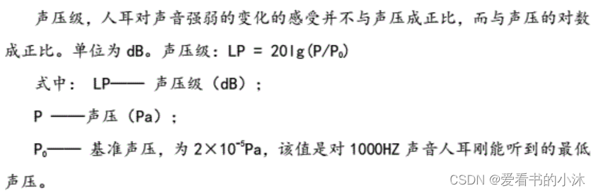
声压级（SPL Sound Pressure Level ）：是指以对数尺衡量有效声压相对于一个基准值的大小，用分贝（dB）来描述其与基准值的关系。人类的对于 1KHz 的声音的听阈（即产生听觉的最低声压）为 20µPa，通常以此作为声压级的基准值。

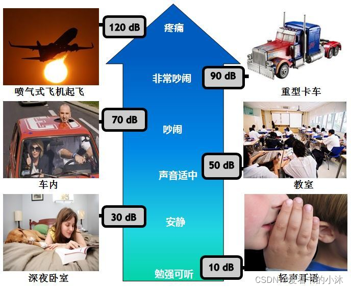
声音测量最常用的物理量是声压，但描述声压的大小通常用声压级（Sound Pressure Level，SPL）。人耳可听的声压范围为2×10^-5Pa到20Pa，对应的声压级范围为0~120dB，因此，引入声压级的概念易于描述线性变化很大的声压。

声压级计算公式：
$$L_p=20\ast lg(\frac{p}{p_0})$$
式中，
Lp:声压级（单位：分贝）；
p：声压（单位：帕）；
p0：基准声压，在空气中 p0=2×10的-5次方（帕），即20微帕 。

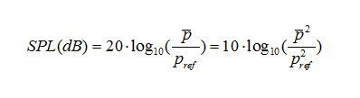
其中，pref表示1000Hz处人耳可听的最小声压幅值20μPa。上式中声压级计算所用的声压p一定是声压的均方根值（RMS），或者是声压的均方值（如果采用10倍的对数形式）。

3、声强

声强：是指单位时间内，声波通过垂直于传播方向单位面积的声能量，用符号I表示，单位为W／m2。声强描述了声能在空间的分布。

声强与声源发射的声功率有关：

• 如果声源在没有边界的自由场向空间发射声波，在离声源半径为r的球面上各点的声强是相同的(此时称为球面波)，且声强与声功率有如下关系：
  $$I=\frac{W}{4\pi \ast r^2}$$

由式可见，若声源发射的声功率不变，声场中各点的声强与距离的平方成反比。

• 如果声源放在地平面上，声波只能向半空间辐射(此时称为平面波)，
  声强与声功率的关系为：
  $$I=\frac{W}{2\pi \ast r^2}$$
• 对于球面波和平面波，声压与声强的关系为：
  $$I=\frac{p^2}{\rho \ast C}$$
  式中，ρ为空气密度，c为声速。
  

4、声功率

声功率：是指单位时间内，声波通过垂直于传播方向某特定面积的声能量，用符号W表示，单位为W。

声压虽然是噪声评价的一个重要物理参量，然而声压的大小与离声源的距离和测量时所处的环境直接相关，所以，不能简单地以声压来衡量一个声源的声辐射能量。而声功率可以用来衡量一个声源的声辐射能力，它是一个恒量。

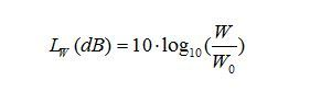
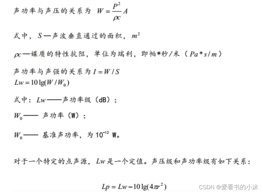
声功率级计算公式:
$$L_w=10\ast lg(\frac{W}{W_0})$$
式中，
Lw：声功率级（单位：分贝）；
W：声功率（单位：瓦）；
W0：基准声功率，W0=10的-12次方（瓦），即1皮瓦。

声能功率不能直接测得,通常测声压换算而得。
声的压强即声强I=p^2/(ρc),或中p为有效声压ρ为空气密度c为空气中的声速。
声功率W=声强x面积
分贝,也称声强级L,表达式是L=lg(I/I0)（式中基准声压I0=10E-12(w/m^2,瓦/平米)。

声功率定义为声源在单位时间内向外辐射的声能，单位为W。与声压级相对应，声功率也存在声功率级。声功率级是声功率与参考声功率的相对量度，定义为

其中W为测量的声功率，W0=10^-12W为基准声功率。声功率是一个绝对量，只与声源有关，与其他无关，因此，它是声源的一个物理属性。

5、时域

时域（时间域，Time domain）是描述数学函数或物理信号对时间的关系。例如一个信号的时域波形可以表达信号随着时间的变化。是真实世界，是惟一实际存在的域。因为我们的经历都是在时域中发展和验证的，已经习惯于事件按时间的先后顺序地发生。而评估数字产品的性能时，通常在时域中进行分析，因为产品的性能最终就是在时域中测量的。

自变量是时间,即横轴是时间,纵轴是信号的变化。其动态信号x（t）是描述信号在不同时刻取值的函数。

时钟波形的两个重要参数是时钟周期和上升时间。

#***********************************************************************
#   Purpose:   绘制时域和频域波形图(单一信号)
#   Author:    爱看书的小沐
#   Date:      2022-02-21 
#   Languages: Python
#   Platform:  Python 3.9.7 win64
# ***********************************************************************
# _*_ coding: utf-8 _*_
from matplotlib import pyplot as plt
import numpy as np

# 中文显示工具函数
def set_params():
    plt.rcParams['font.sans-serif'] = ['FangSong']
    plt.rcParams['axes.unicode_minus'] = False
    fig = plt.figure(figsize=(12, 4))
    fig.canvas.manager.window.wm_geometry('+300+300')

def show_results(x, y, sampling=5):
    n = len(x)
    interval = sampling / n

    # 绘制原始信号的波形图
    ax1 = plt.subplot(2, 1, 1)
    t = np.arange(0, sampling, interval)
    plt.plot(t, x, 'green')
    plt.xlabel('时间（s）'), plt.ylabel('振幅')
    plt.title('(a)原始正弦信号：时域波形图')
    plt.tight_layout()

    # 绘制变换后的波形图
    ax2 = plt.subplot(2, 1, 2)
    frequency = np.arange(n / 2) / (n * interval)
    nfft = abs(y[range(int(n / 2))] / n)
    plt.plot(frequency, nfft, 'red')
    plt.xlabel('频率（Hz）'), plt.ylabel('频谱')
    plt.title(label="(b)傅里叶变换：频域波形图")
    plt.tight_layout()

    # 以动画的方式在上面两幅波形图中同时绘制关键点
    t1 = t[::20]
    val1 = x[::20]
    t2 = frequency[::10]
    val2 = nfft[::10]
    for i in range(0, len(t1)):
        ax1.scatter(t1[i],val1[i], c='b',marker='*') 
        ax2.scatter(t2[i],val2[i], c='b',marker='*') 
        plt.pause(0.1) 

    # 绘制结果图
    plt.show()

if __name__ == "__main__":
    # 生成频率为1，速度为2*pi的正弦波
    time = np.arange(0, 10, .005)
    x = np.sin(2 * np.pi * 1 * time)
    y = np.fft.fft(x)
    set_params()
    show_results(x, y)

6、频域

频域（频率域，frequency domain）是描述信号在频率方面特性时用到的一种坐标系。在电子学，控制系统工程和统计学中，频域图显示了在一个频率范围内每个给定频带内的信号量。频域，尤其在射频和通信系统中运用较多，在高速数字应用中也会遇到频域。频域最重要的性质是：它不是真实的，而是一个数学构造。时域是惟一客观存在的域，而频域是一个遵循特定规则的数学范畴，频域也被一些学者称为上帝视角。

自变量是频率,即横轴是频率,纵轴是该频率信号的幅度,也就是通常说的频谱图。

正弦波是频域中唯一存在的波形，这是频域中最重要的规则，即正弦波是对频域的描述，因为频域中的任何波形都可用正弦波合成。这是正弦波的一个非常重要的性质。

时域分析与频域分析是对模拟信号的两个观察面。时域分析是以时间轴为坐标表示动态信号的关系；频域分析是把信号变为以频率轴为坐标表示出来。一般来说，时域的表示较为形象与直观，频域分析则更为简练，剖析问题更为深刻和方便。信号分析的趋势是从时域向频域发展。然而，它们是互相联系，缺一不可，相辅相成的。

#***********************************************************************
#   Purpose:   绘制时域和频域波形图(两个信号同时叠加)
#   Author:    爱看书的小沐
#   Date:      2022-02-21 
#   Languages: Python
#   Platform:  Python 3.9.7 win64
# ***********************************************************************
# _*_ coding: utf-8 _*_
import numpy as np
import matplotlib.pyplot as plt

def set_params():
    plt.rcParams['font.sans-serif'] = ['FangSong']
    plt.rcParams['axes.unicode_minus'] = False
    fig = plt.figure(figsize=(12, 4))
    fig.canvas.manager.window.wm_geometry('+300+300')

def show_resut():
    sampling_rate = 2000    # 采样率
    fft_size = 1000         # FFT取样长度
    t = np.arange(0, 1, 1.0 / sampling_rate)

    # 两个正弦波叠加，100HZ和50HZ
    x=0.6*np.sin(2*np.pi*100*t)+0.6*np.sin(2*np.pi*50*t)
    xs = x[:fft_size]
    xf = np.fft.rfft(xs) / fft_size  # 返回fft_size/2+1 个频率
    freqs = np.linspace(0, sampling_rate, fft_size//2+1 )  # 表示频率
    xfp = 20 * np.log10(np.clip(np.abs(xf), 1e-20, 1e100))

    # 绘制原始信号的波形图
    ax1 = plt.subplot(211)
    tt = t[:fft_size]
    plt.plot(tt, xs)
    plt.xlabel(u"时间(s)")
    plt.ylabel(u'振幅')
    plt.title(u"100Hz和50Hz的叠加波形的时域图")
    plt.tight_layout()

    # 绘制变换后的波形图
    ax2 = plt.subplot(212)
    plt.plot(freqs, xfp)
    plt.xlabel(u"频率(Hz)")
    plt.ylabel(u'振幅')
    plt.title(u"100Hz和50Hz的叠加波形的频域图")
    plt.tight_layout()

    # 以动画的方式在上面两幅波形图中同时绘制关键点
    t1 = tt[::10]
    val1 = x[::10]
    t2 = freqs[::5]
    val2 = xfp[::5]
    
    print(len(t1), len(t2))
    for i in range(0, len(t1)):
        ax1.scatter(t1[i],val1[i], c='r',marker='*') 
        ax2.scatter(t2[i],val2[i], c='r',marker='*') 
        plt.pause(0.1) 

    # 绘制结果图
    # plt.subplots_adjust(hspace=0.8)
    plt.show()

set_params()
show_resut()

7、时频域

时频分布是一项让我们能够同时观察一个讯号的时域和频域资讯的工具，而时频分析就是在分析时频分布。传统上，我们常用傅里叶变换来观察一个讯号的频谱。然而，这样的方法不适合用来分析一个频率会随着时间而改变的讯号。

• （1）基于MATLAB的短时傅里叶变换函数：spectrogram
  https://www.mathworks.com/help/signal/ref/spectrogram.html
  3D Spectrogram Visualization：Generate two seconds of a signal sampled at 10 kHz. Specify the instantaneous frequency of the signal as a triangular function of time. Spectrogram() using short-time Fourier transform.

fs = 10e3;
t = 0:1/fs:2;
x1 = vco(sawtooth(2*pi*t,0.5),[0.1 0.4]*fs,fs);
spectrogram(x1,kaiser(256,5),220,512,fs,'yaxis')

view(-45,65)
colormap bone

• （2）基于Python实现的2d绘制时频图
  https://docs.scipy.org/doc/scipy/reference/generated/scipy.signal.chirp.html?highlight=spectrogram

#***********************************************************************
#   Purpose:   绘制2d时频图（基于chirp信号）
#   Author:    爱看书的小沐
#   Date:      2022-02-21 
#   Languages: Python
#   Platform:  Python 3.9.7 win64
# ***********************************************************************
from scipy.signal import chirp, spectrogram
import matplotlib.pyplot as plt
import matplotlib.animation as animation
import numpy as np

# define vars
fig = plt.figure(figsize=(12, 4))
fs = 150
T = 4
t = np.arange(0, int(T*fs)) / fs
w = chirp(t, f0=20, f1=10, t1=T, method='linear')

def plot_spectrogram(title, w, fs):
    ff, tt, Sxx = spectrogram(w, fs=fs, nperseg=64, nfft=256)
    plt.pcolormesh(tt, ff[:145], Sxx[:145], cmap='gray_r', shading='gouraud')
    plt.title(title)
    plt.xlabel('t (sec)')
    plt.ylabel('Frequency (Hz)')
    plt.grid()

# plot 1
ax1 = plt.subplot(211)
plot_spectrogram(f'spectrogram: Linear Chirp, f(0)=20, f({T})=10', w, fs)
plt.tight_layout()

# plot 2
ax2 = plt.subplot(212, sharex=ax1)
plt.plot(t, w, color='blue')
plt.title(f"plot: Linear Chirp, f(0)=20, f({T})=10")
plt.xlabel('t (sec)')
plt.ylabel('Amplitude')
plt.tight_layout()

# plot 2 by animation
def update_points(num):
    point_ani.set_data(t[num], w[num])
    if num % 5 == 0:
        point_ani.set_marker("*")
        point_ani.set_markersize(8)
    else:
        point_ani.set_marker("o")
        point_ani.set_markersize(4)
 
    text_pt.set_position((t[num], w[num]))
    text_pt.set_text("x=%.3f, y=%.3f" % (t[num], w[num]))
    return point_ani, text_pt,

point_ani, = plt.plot(t[0], w[0], "ro")
plt.grid(ls="--")
text_pt = plt.text(4, 0.8, '', fontsize=10)
ani = animation.FuncAnimation(fig, update_points, np.arange(0, 100), interval=300, blit=True)
ani.save('test.gif', writer='Pillow', fps=10)

# show results
plt.show()

• （3）基于Python实现的3d绘制时频图

#***********************************************************************
#   Purpose:   绘制3d时频图（基于chirp信号）
#   Author:    爱看书的小沐
#   Date:      2022-02-21 
#   Languages: Python
#   Platform:  Python 3.9.7 win64
# ***********************************************************************
import numpy as np
import pandas as pd
import numpy as np
from scipy import signal
import matplotlib.pyplot as plt
from mpl_toolkits.mplot3d import Axes3D
from matplotlib import cm
from matplotlib.collections import PolyCollection
from matplotlib import mlab
import matplotlib.pyplot as plt
import numpy as np

from matplotlib import animation

# Fixing random state for reproducibility
np.random.seed(666)

title = ('2 Vrms sine wave with modulated frequency around 3kHz, '
         'corrupted by white noise of exponentially decreasing '
         'magnitude sampled at 10 kHz.')

# Define vars
# fs = 10e3
fs = 100
# N = 1e5
N = 1e4
amp = 2 * np.sqrt(2)
noise_power = 0.01 * fs / 2
t = np.arange(N) / float(fs)
mod = 500*np.cos(2*np.pi*0.25*t)
carrier = amp * np.sin(2*np.pi*3e3*t + mod)
noise = np.random.normal(scale=np.sqrt(noise_power), size=t.shape)
noise *= np.exp(-t/5)
y = carrier + noise

# Define plot 2d
def specgram2d(y, srate=44100, ax=None, title=None):
  if not ax:
    ax = plt.axes()
  ax.set_title(title, loc='center', wrap=True, fontdict={'weight':'normal','size': 8})
  spec, freqs, t, im = ax.specgram(y, Fs=fs, scale='dB', vmax=0)
  ax.set_xlabel('time (s)')
  ax.set_ylabel('frequencies (Hz)')
  cbar = plt.colorbar(im, ax=ax)
  cbar.set_label('Amplitude (dB)')
  cbar.minorticks_on()
  return spec, freqs, t, im

# Define plot 3d
def specgram3d(y, srate=44100, ax=None, title=None):
  if not ax:
    ax = plt.axes(projection='3d')
  ax.set_title(title, loc='center', wrap=True)
  spec, freqs, t = mlab.specgram(y, Fs=srate)
  X, Y, Z = t[None, :], freqs[:, None],  20.0 * np.log10(spec)
  ax.plot_surface(X, Y, Z, cmap='viridis')
  ax.set_xlabel('time (s)')
  ax.set_ylabel('frequencies (Hz)')
  ax.set_zlabel('amplitude (dB)')
  ax.set_zlim(-80, 0)
  return X, Y, Z

# Call plot 2d 
fig = plt.figure(figsize=(12, 4))
ax1 = plt.subplot(121)
specgram2d(y, srate=fs, title=title, ax = ax1)
plt.tight_layout()

# Call plot 3d 
ax2 = plt.subplot(122, projection= "3d")
specgram3d(y, srate=fs, title="", ax = ax2)
plt.tight_layout()

# Animate plot 3d
def animate(i):
    ax2.view_init(azim=i)
rot_animation = animation.FuncAnimation(fig, animate, frames=np.arange(0,360+2,2), interval=100)
rot_animation.save('test.gif', writer='pillow')

plt.show()

• （3）基于Python实现的绘制WAV声音文件的时频图

#***********************************************************************
#   Purpose:   绘制wav声音文件时频图
#   Author:    爱看书的小沐
#   Date:      2022-02-21 
#   Languages: Python
#   Platform:  Python 3.9.7 win64
# ***********************************************************************

import matplotlib.pyplot as plt
import numpy as np
from scipy.io import wavfile
from matplotlib import animation

fig = plt.figure(figsize=(12, 6))
fig.canvas.manager.window.wm_geometry('+150+150')

#################################################################################
# Read the wav file (mono)
samplingFrequency, signalData = wavfile.read('d:\wind.wav')
print(samplingFrequency, len(signalData))
 
# Plot the signal read from wav file
ax221 = plt.subplot(221)
plt.title('Spectrogram of a wav file with single-channel music')
plt.plot(signalData)
plt.xlabel('Sample')
plt.ylabel('Amplitude')
plt.grid(ls="--")
plt.tight_layout()

point_221, = plt.plot(signalData, "bo")
text_221 = plt.text(4, 0.8, '', fontsize=10)

plt.subplot(222)
plt.specgram(signalData,Fs=samplingFrequency)
plt.xlabel('Time')
plt.ylabel('Frequency')
plt.tight_layout()

#################################################################################
# Define the list of frequencies
frequencies         = np.arange(5,105,5)

# Sampling Frequency
samplingFrequency   = 400

# Create two ndarrays
s1 = np.empty([0])  # For samples
s2 = np.empty([0])  # For signal

# Start Value of the sample
start   = 1

# Stop Value of the sample
stop    = samplingFrequency+1

for frequency in frequencies:
    sub1 = np.arange(start, stop, 1)

    # Signal - Sine wave with varying frequency + Noise
    sub2 = np.sin(2*np.pi*sub1*frequency*1/samplingFrequency)+np.random.randn(len(sub1))
    s1      = np.append(s1, sub1)
    s2      = np.append(s2, sub2)
    start   = stop+1
    stop    = start+samplingFrequency

# Plot the signal
plt.subplot(223, sharex=ax221)
plt.title('Spectrogram of signal in frequency domain')
plt.plot(s1,s2)
plt.grid(ls="--")
plt.xlabel('Sample')
plt.ylabel('Amplitude')
plt.tight_layout()

point_223, = plt.plot(s1[0], s2[0], "ro" )
text_223 = plt.text(4, 0.8, '', fontsize=10)

# Plot the spectrogram
plt.subplot(224)
powerSpectrum, freqenciesFound, time, imageAxis = plt.specgram(s2, Fs=samplingFrequency)
plt.xlabel('Time')
plt.ylabel('Frequency')
plt.tight_layout()

#################################################################################
# Animate 
def update_points(num):
    point_221.set_data(num, signalData[num])
    point_223.set_data(s1[num], s2[num])

    if num % 10 == 0:
        point_221.set_marker("*")
        point_221.set_markersize(8)
        point_223.set_marker("*")
        point_223.set_markersize(8)
    else:
        point_221.set_marker("o")
        point_221.set_markersize(6)
        point_223.set_marker("o")
        point_223.set_markersize(6)
 
    text_221.set_position((num, signalData[num]))
    text_221.set_text("x=%d, y=%.3f" % (num, signalData[num]))
    text_223.set_position((s1[num], s2[num]))
    text_223.set_text("x=%.3f, y=%.3f" % (s1[num], s2[num]))
    return point_223, text_223,point_221, text_221,

ani = animation.FuncAnimation(fig, update_points, np.arange(0, len(s1)), interval=100, blit=True)
# ani.save('test2.gif', writer='Pillow', fps=10)

plt.show()   

8、空域

空域（空间域，spatial domain），又称图像空间(image space)，一般这个概念会出现在数字图像处理中，指由图像像元组成的空间。在图像空间中以长度(距离)为自变量直接对像元值进行处理称为空间域处理。

9、压力声学

压力声学是“声学模块”最常用的功能，可以用于模拟压力声学效应，例如声音的散射、衍射、发射、辐射和传输。在频域中运行的仿真使用亥姆霍兹方程，而时域仿真则使用经典的标量波动方程。在频域中，您可以使用有限元法和边界元法，以及混合有限元-边界元法。在时域中，可以使用时域隐式（有限元法）和时域显式（dG-FEM）公式。

结语

如果您觉得该方法或代码有一点点用处，可以给作者点个赞，或打赏杯咖啡；╮(￣▽￣)╭
如果您感觉方法或代码不咋地//(ㄒoㄒ)//，就在评论处留言，作者继续改进；o_O???
如果您需要相关功能的代码定制化开发，可以留言私信作者；(✿◡‿◡)
感谢各位大佬童鞋们的支持！( ´ ▽´ )ﾉ ( ´ ▽´)っ！！！