凸优化第七章统计估计作业题

最新推荐文章于 2021-07-13 09:00:55 发布

使君杭千秋

最新推荐文章于 2021-07-13 09:00:55 发布

阅读量418

点赞数 1

分类专栏：凸优化

原文链接：https://blog.csdn.net/wangchy29/article/details/87474818

版权

凸优化专栏收录该内容

62 篇文章 47 订阅

订阅专栏

极大似然估计

Let $x^{(1)}\cdots x^{(N)}$ be independent samples from an N(μ,Σ) distribution, where it is known that $\Sigma ^{min} \leq \Sigma \leq \Sigma^{max}$ , where $\Sigma^{min}$ and $\Sigma^{max}$ are given positive definite matrices. Which of the following is true?

最优检测器设计

Consider a binary detection system with the following confusion matrix

$D = \left[\begin{array}{ll} 0.75 & 0.15 \\ 0.25 & 0.85 \end{array} \right ].$

If both classes are equiprobable, what is the probability of error

错误的概率，即实际是假设1成立，而估计为假设2，以及实际是假设2而估计为假设1。一直每种假设发生的概率均为0.5，故错误的概率= 0.1*-。25+0.15*0.5=0.2

In binary hypothesis testing the likelihood ratio threshold can be interpreted as the cost of misclassification.

实验设计

If you solve the relaxed version of the optimal experiment design problem, and then simply round to get the (integer) number of times to carry out each experiment, you get the globally optimal (integer) experiment design.

Maximum likelihood estimation of an increasing nonnegative signal

We wish to estimate a scalar signal x(t), for t=1,2,…,N, which is known to be nonnegative and monotonically nondecreasing:

$0 \leq x(1) \leq x(2) \leq \cdots \leq x(N).$

This occurs in many practical problems. For example, x(t) might be a measure of wear or deterioration, that can only get worse, or stay the same, as time t increases. We are also given that x(t)=0 for t≤0.

We are given a noise-corrupted moving average of x, given by

$y(t) = \sum_{\tau=1}^k h(\tau) x(t-\tau) + v(t),\quad t=2, \ldots, N+1,$

where v(t) are independent N(0,1) random variables.

Formulate the problem of finding the maximum likelihood estimate of x, given y, taking into account the prior assumption that x is nonnegative and monotonically nondecreasing, as a convex optimization problem. Now solve a specific instance of the problem, with problem data (i.e., N, k, h, and y) given in the file ml_estim_incr_signal_data_norng.m. (This file contains the true signal xtrue, which of course you cannot use in creating your estimate.) Find the maximum likelihood estimate x^ml, and plot it, along with the true signal. Also find and plot the maximum likelihood estimate x^ml,free not taking into account the signal nonnegativity and monotonicity.

Hint. The function conv (convolution) is overloaded to work with CVX.

Which of the following statements most accurately describe the plot

Worst-case probability of loss

Two investments are made, with random returns $R_1$ and $R_2$ .The total return for the two investments is $R_1+R_2$ , and the probability of a loss (including breaking even, i.e., $R_1+R_2=0$ ) is ploss=prob( $R_1+R_2\leq 0$ ). The goal is to find the worst-case (i.e., maximum possible) value of ploss, consistent with the following information. Both $R_1$ and $R_2$ have Gaussian marginal distributions, with known means $\mu _1$ and $\mu_2$ and known standard deviations $\delta_1$ and $\delta _2$ . In addition, it is known that $R_1$ and $R_2$ are correlated with correlation coefficient ρ, i.e.,

$\mathbf{E} (R_1-\mu_1) (R_2-\mu_2) = \rho \sigma_1 \sigma_2.$

Your job is to find the worst-case ploss over any joint distribution of $R_1$ and $R_2$ consistent with the given marginals and correlation coefficient.

We will consider the specific case with data

$\mu_1 = 8, \quad \mu_2 = 20, \quad \sigma_1 = 6, \quad \sigma_2 = 17.5,\quad \rho = -0.25.$

We can compare the results to the case when $R_1$ and $R_2$ are jointly Gaussian. In this case we have

$R_1+R_2 \sim \mathcal N(\mu_1+\mu_2,\sigma_1^2+\sigma_2^2+2 \rho \sigma_1\sigma_2),$

which for the data given above gives $p^\mathrm{loss} = 0.050$ . Your job is to see how much larger $p^\mathrm{loss}$ can possibly be.

This is an infinite-dimensional optimization problem, since you must maximize $p^\mathrm{loss}$ over an infinite-dimensional set of joint distributions. To (approximately) solve it, we discretize the values that $R_1$ and $R_2$ can take on, to n=100 values r1,…,rn, uniformly spaced from $r_1=-30$ to $r_n=+70$ . We use the discretized marginals $p^{(1)}$ and $p^{(2)}$ for $R_1$ and $R_2$ , given by

$p^{(k)}_i =\mathbf{prob}(R_k = r_i) =\frac{ \exp \left(-(r_i-\mu_k)^2/(2 \sigma_k^2) \right)}{\sum_{j=1}^n \exp \left( -(r_j-\mu_k)^2/(2 \sigma_k^2) \right)},$

for k=1,2, i=1,…,n.

Formulate the (discretized) problem as a convex optimization problem, and solve it. What is the maximum value of ploss?

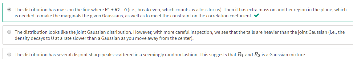
Plot the joint distribution that yields the maximum value of ploss using the Matlab commands mesh and contour. Which of the following statements most accurately describe the plot of the (worst-case) joint distribution?

来源：https://blog.csdn.net/wangchy29/article/details/87474818

使君杭千秋

关注

1
点赞
踩
0

收藏

觉得还不错? 一键收藏
1
评论
凸优化第七章统计估计作业题

极大似然估计Letbe independent samples from anN(μ,Σ)distribution, where it is known that, whereandare given positive definite matrices. Which of the following is true?最优检测器设计Consider a binary detection system with the following confusion matrix...
复制链接

扫一扫