


sklearn.ensemble模块包括两个基于随机决策树的算法:随机森林算法和树外方法。这些算法是特别对于树的扰动与结合技术。这就意味着多种分类器的集合通过在分类器构建过程中引入随机项而被构建。这种集成的预测通过个体的分类的平均预测。
像其它分类器一样,森林分类器必须拟合两个矩阵:大小为[n_samples, n_features]的X(包含训练样本),大小为[n_samples]的Y,包含训练样本的目标值。
1.随机森林
在随机森林中,集成中的每一棵树都是由样本有放回地抽出来,此外当在构建树的过程中切割节点时,不再是对于所有特征的最优切割点,而是随机特征子集中的最优切割节点。由于这种随机性,森林的偏差通常会略微增加(相对于单个非随机树),但是由于平均化,它的方差也减小了,通常对于偏差的这种补偿会产生更好的模型。
与先前的研究相反,sklearn编译器通过结合平均化概率的预测,而不是通过对每个学习器投票得到结果。
2.极端随机树
在极端随机树(ExtraTreesClassifier和 ExtraTreesRegressor)中,随机化往前走了一步,它的切割点是被计算的。就像在随机森林中一样,候选特征的随机子集被使用,而不是去找最差异化的阈值,阈值对于每个候选特征被随机引入,这些随机产生的阈值最优的被选择作为切割规则。这通常允许减少多一点的模型方差(以增加偏差为代价)。
print(__doc__)

import numpy as np
import matplotlib.pyplot as plt

from sklearn import clone
from sklearn.datasets import load_iris
from sklearn.ensemble import (RandomForestClassifier, ExtraTreesClassifier,
                              AdaBoostClassifier)
from sklearn.externals.six.moves import xrange
from sklearn.tree import DecisionTreeClassifier

# Parameters
n_classes = 3
n_estimators = 30
plot_colors = "ryb"
cmap = plt.cm.RdYlBu
plot_step = 0.02  # fine step width for decision surface contours
plot_step_coarser = 0.5  # step widths for coarse classifier guesses
RANDOM_SEED = 13  # fix the seed on each iteration

# Load data
iris = load_iris()

plot_idx = 1

models = [DecisionTreeClassifier(max_depth=None),
          RandomForestClassifier(n_estimators=n_estimators),
          ExtraTreesClassifier(n_estimators=n_estimators),
          AdaBoostClassifier(DecisionTreeClassifier(max_depth=3),
                             n_estimators=n_estimators)]

for pair in ([0, 1], [0, 2], [2, 3]):
    for model in models:
        # We only take the two corresponding features
        X = iris.data[:, pair]
        y = iris.target

        # Shuffle
        idx = np.arange(X.shape[0])
        np.random.seed(RANDOM_SEED)
        np.random.shuffle(idx)
        X = X[idx]
        y = y[idx]

        # Standardize
        mean = X.mean(axis=0)
        std = X.std(axis=0)
        X = (X - mean) / std

        # Train
        clf = clone(model)
        clf = model.fit(X, y)

        scores = clf.score(X, y)
        # Create a title for each column and the console by using str() and
        # slicing away useless parts of the string
        model_title = str(type(model)).split(".")[-1][:-2][:-len("Classifier")]
        model_details = model_title
        if hasattr(model, "estimators_"):
            model_details += " with {} estimators".format(len(model.estimators_))
        print( model_details + " with features", pair, "has a score of", scores )

        plt.subplot(3, 4, plot_idx)
        if plot_idx <= len(models):
            # Add a title at the top of each column
            plt.title(model_title)

        # Now plot the decision boundary using a fine mesh as input to a
        # filled contour plot
        x_min, x_max = X[:, 0].min() - 1, X[:, 0].max() + 1
        y_min, y_max = X[:, 1].min() - 1, X[:, 1].max() + 1
        xx, yy = np.meshgrid(np.arange(x_min, x_max, plot_step),
                             np.arange(y_min, y_max, plot_step))

        # Plot either a single DecisionTreeClassifier or alpha blend the
        # decision surfaces of the ensemble of classifiers
        if isinstance(model, DecisionTreeClassifier):
            Z = model.predict(np.c_[xx.ravel(), yy.ravel()])
            Z = Z.reshape(xx.shape)
            cs = plt.contourf(xx, yy, Z, cmap=cmap)
        else:
            # Choose alpha blend level with respect to the number of estimators
            # that are in use (noting that AdaBoost can use fewer estimators
            # than its maximum if it achieves a good enough fit early on)
            estimator_alpha = 1.0 / len(model.estimators_)
            for tree in model.estimators_:
                Z = tree.predict(np.c_[xx.ravel(), yy.ravel()])
                Z = Z.reshape(xx.shape)
                cs = plt.contourf(xx, yy, Z, alpha=estimator_alpha, cmap=cmap)

        # Build a coarser grid to plot a set of ensemble classifications
        # to show how these are different to what we see in the decision
        # surfaces. These points are regularly space and do not have a black outline
        xx_coarser, yy_coarser = np.meshgrid(np.arange(x_min, x_max, plot_step_coarser),
                                             np.arange(y_min, y_max, plot_step_coarser))
        Z_points_coarser = model.predict(np.c_[xx_coarser.ravel(), yy_coarser.ravel()]).reshape(xx_coarser.shape)
        cs_points = plt.scatter(xx_coarser, yy_coarser, s=15, c=Z_points_coarser, cmap=cmap, edgecolors="none")

        # Plot the training points, these are clustered together and have a
        # black outline
        for i, c in zip(xrange(n_classes), plot_colors):
            idx = np.where(y == i)
            plt.scatter(X[idx, 0], X[idx, 1], c=c, label=iris.target_names[i],
                        cmap=cmap)

        plot_idx += 1  # move on to the next plot in sequence

plt.suptitle("Classifiers on feature subsets of the Iris dataset")
plt.axis("tight")

plt.show()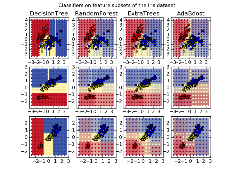
画出iris数据集特征对的训练随机树的森林决策平面。
这个图比较了被一个决策树分类器(第一列)学习到的决策平面,以及随机森林、树外分类器还有AdaBoost结果。
第一行分类器使用萼片宽度和长度作为特征,第二行使用花瓣长度和萼片长度,第三行使用花瓣宽度和花瓣长度。
按照质量递减的顺序,当对于所有4个特征使用30个学习器训练的时候使用10折交叉验证,我们可以得到
ExtraTreesClassifier()  # 0.95 score
RandomForestClassifier()  # 0.94 score
AdaBoost(DecisionTree(max_depth=3))  # 0.94 score
DecisionTree(max_depth=None)  # 0.94 score
增加AdaBoost 的最大深度降低了得分的标准差,但是平均得分并没有增加。
对于提高模型,我们可以尝试:
1.DecisionTreeClassifier 和 AdaBoostClassifier可以改变max_depth,可以产生尝试max_depth=3(DecisionTreeClassifier)以及depth=None(max_depth=None)
2.改变n_estimators。
值得注意的是,RandomForests 和 ExtraTrees每棵树可以独立跑,因此可以多核并行。而 AdaBoost是序列型建立,不能使用多核。
3.参数
主要参数就是n_estimators 和max_features。前者是森林中树的个数,越大越好当然也越费计算时间。此外,当结果超过树的临界数时,结果将不会变得更好。后者是当切割点是要考虑的特征的随机子集的大小。方差越低越好,但也会使得偏差增大。经验上来说对于回归问题max_features=n_features,对于分类问题max_features=sqrt(n_features),其中n_features是数据特征的个数。比较好的结果通常设置成max_depth=None以及min_samples_split=1相结合的方式。注意这些结果通常来说的不是最佳的,可能造成很耗内存。最优的参数总是应该被交叉验证。此外,注意,random forests,和bootstrap默认bootstrap=True,而extra-trees默认设置bootstrap=False。单数用bootstrap时,可以通过oob_score=True计算泛化误差。
4.并行
最后,模块通过n_jobs参数作为预测并行计算的特征。如果n_jobs=k,则被分成在k个核上的k个线程跑。如果n_jobs=-1,则在所有可用的核上。注意,由于内部管道的交互处理,这种加速也许不是线性的(也就是说k核跑不一定会使速度提高k倍)。在大量树的情况下这种加速还是很显著的。
References
L.Breiman, “Random Forests”, Machine Learning, 45(1), 5-32, 2001.
L.Breiman, “Arcing Classifiers”, Annals of Statistics 1998.
[GEW2006] P. Geurts, D. Ernst., and L. Wehenkel, “Extremely randomized trees”, Machine Learning, 63(1), 3-42, 2006.
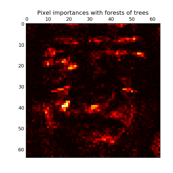
5.特征重要性评估
一个在树中被使用作为决策节点的特征的相对排名可以被用来评估这个特征相对于目标变量的特征的相对重要性。在树顶端被使用的特征决定了大部分样本输入的最后预测结果。它们所起作用的样本的期望比例因此可以被使用作为特征相对重要性的估计。
通过平均化这些随机树的期望活性率,可以减少这些学习器的方差并且使用它来作特征筛选。
接下来的例子展示了图像分类中通过树的森林的每个像素点的重要性,其中像素点越热表明越重要。
print(__doc__)

from time import time
import matplotlib.pyplot as plt

from sklearn.datasets import fetch_olivetti_faces
from sklearn.ensemble import ExtraTreesClassifier

# Number of cores to use to perform parallel fitting of the forest model
n_jobs = 1

# Load the faces dataset
data = fetch_olivetti_faces()
X = data.images.reshape((len(data.images), -1))
y = data.target

mask = y < 5  # Limit to 5 classes
X = X[mask]
y = y[mask]

# Build a forest and compute the pixel importances
print("Fitting ExtraTreesClassifier on faces data with %d cores..." % n_jobs)
t0 = time()
forest = ExtraTreesClassifier(n_estimators=1000,
                              max_features=128,
                              n_jobs=n_jobs,
                              random_state=0)

forest.fit(X, y)
print("done in %0.3fs" % (time() - t0))
importances = forest.feature_importances_
importances = importances.reshape(data.images[0].shape)

# Plot pixel importances
plt.matshow(importances, cmap=plt.cm.hot)
plt.title("Pixel importances with forests of trees")
plt.show()
6. Totally Random Trees Embedding
随机树嵌入实施了一个非监督的数据转化。使用完全随机树的一个森林,RandomTreesEmbedding通过索引留出一个数据终止。这个索引然后通过K个方式中的一个编码,得到高维稀疏二进制编码。这种编码可以被非常高效地计算,然后被用来作为其它学习任务的基础。这种编码的大小和稀疏性可以通过选择树的数量和每棵树的深度来影响。对于每一棵集成中的树,这种编码包含每棵树一个号。编码的大小是至多n_estimators * 2 ** max_depth,森林中叶子数的最大值。
由于临近数据的点通常都落在一棵树的相同叶子上,这种转换执行的就非常明确,没有参数密度估计。
example: Hashing feature transformation using Totally Random Trees

RandomTreesEmbedding提供了一种将数据map到一个高维稀疏的表示,这样有利于分类。这种mapping完全无监督并且非常高效。
这个例子给定了一些树的分开部分的可视化,展示了这种转化如何被用来进行非线性的降维或者非线性分类。
这些临近的点在树中共享相同的叶子,因此共享了大部分的hash表示。这允许分开两个同心圆基于转化数据的主成分分析。
在高维空间中,线性分类器通常都会实现杰出的准确率。对于稀疏的二进制数据,BernoulliNB 部分适配很好。底部一行比较了BernoulliNB得到的在转化数据空间中的决定边界以及原始数据中学习到的ExtraTreesClassifier森林。
import numpy as np
import matplotlib.pyplot as plt

from sklearn.datasets import make_circles
from sklearn.ensemble import RandomTreesEmbedding, ExtraTreesClassifier
from sklearn.decomposition import TruncatedSVD
from sklearn.naive_bayes import BernoulliNB

# make a synthetic dataset
X, y = make_circles(factor=0.5, random_state=0, noise=0.05)

# use RandomTreesEmbedding to transform data
hasher = RandomTreesEmbedding(n_estimators=10, random_state=0, max_depth=3)
X_transformed = hasher.fit_transform(X)

# Visualize result using PCA
pca = TruncatedSVD(n_components=2)
X_reduced = pca.fit_transform(X_transformed)

# Learn a Naive Bayes classifier on the transformed data
nb = BernoulliNB()
nb.fit(X_transformed, y)


# Learn an ExtraTreesClassifier for comparison
trees = ExtraTreesClassifier(max_depth=3, n_estimators=10, random_state=0)
trees.fit(X, y)


# scatter plot of original and reduced data
fig = plt.figure(figsize=(9, 8))

ax = plt.subplot(221)
ax.scatter(X[:, 0], X[:, 1], c=y, s=50)
ax.set_title("Original Data (2d)")
ax.set_xticks(())
ax.set_yticks(())

ax = plt.subplot(222)
ax.scatter(X_reduced[:, 0], X_reduced[:, 1], c=y, s=50)
ax.set_title("PCA reduction (2d) of transformed data (%dd)" %
             X_transformed.shape[1])
ax.set_xticks(())
ax.set_yticks(())

# Plot the decision in original space. For that, we will assign a color to each
# point in the mesh [x_min, m_max] x [y_min, y_max].
h = .01
x_min, x_max = X[:, 0].min() - .5, X[:, 0].max() + .5
y_min, y_max = X[:, 1].min() - .5, X[:, 1].max() + .5
xx, yy = np.meshgrid(np.arange(x_min, x_max, h), np.arange(y_min, y_max, h))

# transform grid using RandomTreesEmbedding
transformed_grid = hasher.transform(np.c_[xx.ravel(), yy.ravel()])
y_grid_pred = nb.predict_proba(transformed_grid)[:, 1]

ax = plt.subplot(223)
ax.set_title("Naive Bayes on Transformed data")
ax.pcolormesh(xx, yy, y_grid_pred.reshape(xx.shape))
ax.scatter(X[:, 0], X[:, 1], c=y, s=50)
ax.set_ylim(-1.4, 1.4)
ax.set_xlim(-1.4, 1.4)
ax.set_xticks(())
ax.set_yticks(())

# transform grid using ExtraTreesClassifier
y_grid_pred = trees.predict_proba(np.c_[xx.ravel(), yy.ravel()])[:, 1]

ax = plt.subplot(224)
ax.set_title("ExtraTrees predictions")
ax.pcolormesh(xx, yy, y_grid_pred.reshape(xx.shape))
ax.scatter(X[:, 0], X[:, 1], c=y, s=50)
ax.set_ylim(-1.4, 1.4)
ax.set_xlim(-1.4, 1.4)
ax.set_xticks(())
ax.set_yticks(())

plt.tight_layout()
plt.show()


 1302
1302


 被折叠的 条评论
为什么被折叠?
被折叠的 条评论
为什么被折叠?
 到【灌水乐园】发言


