多元线性回归

多元线性回归

---

• 符号解释：

$n$：特征的个数
$x^{(i)}$：第i个训练样本
$x_j^{(i)}$：第$i$个训练样本的第$j$个特征值

预测函数：
$$h_{\theta }(x)={\theta }_0+{\theta }_1{x}_1+{\theta }_2{x}_2+...+{\theta }_n{x}_n$$
为了方便，我们定义$x_0=1$
$$x=\left[\begin{array}{c}{x}_0\\ x_1\\ x_2\\ ⋮\\ x_n\end{array}\right]$$

$$\theta =\left[\begin{array}{c}{\theta }_0\\ {\theta }_1\\ {\theta }_2\\ ⋮\\ {\theta }_n\end{array}\right]$$

则有$$h_{\theta }(x)={\theta }_0{x}_0+{\theta }_1{x}_1+{\theta }_2{x}_2+...+{\theta }_n{x}_n$$
$$={\theta }^T\cdot x$$

多元梯度下降

---

预测函数：$$h_{\theta }(x)={\theta }^T\cdot x={\theta }_0{x}_0+{\theta }_1{x}_1+{\theta }_2{x}_2+...+{\theta }_n{x}_n$$
代价函数：$$J({\theta }_0,{\theta }_1,\dots ,{\theta }_n)=\frac{1}{2m}\sum _{i=1}^m(h_{\theta }(x^{(i)})-y^{(i)}{)}^2$$

梯度下降算法：

R e p e a t {                                                              Repeat\{ \ \ \ \ \ \ \ \ \ \ \ \ \ \ \ \ \ \ \ \ \ \ \ \ \ \ \ \ \ \ \ \ \ \ \ \ \ \ \ \ \ \ \ \ \ \ \ \ \ \ \ \ \ \ \ \ \ \ \ \ Repeat{                                                            
$${\theta }_j:={\theta }_j-\alpha \frac{\partial }{\partial {\theta }_j}J({\theta }_0,{\theta }_1,\dots ,{\theta }_n)forj=0,1,\dots ,n$$
$$\}$$


求导得：
R e p e a t {                                                              Repeat\{ \ \ \ \ \ \ \ \ \ \ \ \ \ \ \ \ \ \ \ \ \ \ \ \ \ \ \ \ \ \ \ \ \ \ \ \ \ \ \ \ \ \ \ \ \ \ \ \ \ \ \ \ \ \ \ \ \ \ \ \ Repeat{                                                            
$${\theta }_j:={\theta }_j-\alpha \frac{1}{m}\sum _{i=1}^m(h_{\theta }(x^{(i)})-y^{(i)})\cdot x_j^{(i)}$$
$$\}$$

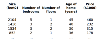
梯度下降法实践1：特征缩放

---

在我们面对多维特征问题的时候，我们要保证这些特征都具有相近的尺度，这将帮助梯
度下降算法更快地收敛。

比如以房价问题为例，假设我们使用两个特征，房屋的尺寸和房间的数量，尺寸的值为 0
2000 平方英尺，而房间数量的值则是 0-5，以两个参数分别为横纵坐标，绘制代价函数的等
高线图能，看出图像会显得很扁，梯度下降算法需要非常多次的迭代才能收敛。

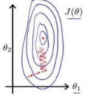
特征缩放是一种有效的解决方法：尝试将所有特征的尺度都尽量缩放到-1 到 1 之间。如图：

最简单的方法是令$$x_n=\frac{x_n-{\mu }_n}{s_n}$$

其中，${\mu }_n$是平均值，$s_n$是标准差，或者极差（最大值减最小值）。

梯度下降法实践2: 学习率$\alpha$

---

梯度下降算法收敛所需要的迭代次数根据模型的不同而不同，我们不能提前预知，我们
可以绘制迭代次数和代价函数的图表来观测算法需要几次迭代趋于收敛。

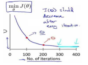
$J(\theta )$应该在每次迭代后都减少。
我们也可以设置：当一次迭代后减少的值小于特定阈值时停止。

梯度下降算法的每次迭代受到学习率的影响

• 如果学习率?过小，则达到收敛所需的迭代次数会非常高；
• 如果学习率?过大，每次迭代可能不会减小代价函数，可能会越过局部最小值导致无法收敛。

通常使用这些学习率：
? = 0.01，0.03，0.1，0.3，1，3，10

Python代码实现

---

import numpy as np
import matplotlib.pyplot as plt
import pandas as pd
import seaborn as sns

df = pd.read_csv('ex1data2.txt', names=['size', 'rooms', 'price'])
# print(df.head())


def normalize_feature(df):
    return df.apply(lambda column: (column - column.mean()) / column.std())#特征缩放


df = normalize_feature(df)


def get_X(df):
    ones = pd.DataFrame({'ones': np.ones(len(df))})
    data = pd.concat([ones, df], axis=1)
    return data.iloc[:, :-1].as_matrix()


def get_y(df):
    return np.array(df.iloc[:, -1].as_matrix())


X = get_X(df)
y = get_y(df)
m = X.shape[0]
n = X.shape[1]
theta = np.zeros(n)


def lr_cost(theta, X, y):
    inner = (X.dot(theta) - y)
    cost = inner.T.dot(inner)
    return cost/(2 * m)


def gradient(theta, X, y):
    inner = X.T.dot(X.dot(theta) - y)
    return inner/m


def batch_gradient(theta, X, y, epoch, alpha=0.01):
    _theta = theta.copy()
    cost_data = [lr_cost(theta, X, y)]
    for _ in range(epoch):
        _theta = _theta - alpha * gradient(_theta, X, y)
        cost_data.append(lr_cost(_theta, X, y))
    return _theta, cost_data


epoch = 500
final_theta, cost_data = batch_gradient(theta, X, y, epoch)
print(final_theta)
sns.tsplot(time=np.arange(len(cost_data)), data=cost_data)
plt.xlabel('epoch', fontsize=18)
plt.ylabel('cost', fontsize=18)
plt.show()