


1. 感知机
在机器学习中,感知机(Perceptron)是二分类的线性分类模型,属于监督学习算法。输入为实例的特征向量,输出为实例的类别(取+1和-1)。感知机对应于输入空间中将实例划分为两类的分离超平面。感知机旨在求出该超平面,为求得超平面导入了基于误分类的损失函数,利用随机梯度下降法(SGD)对损失函数进行最优化。
2. 感知机python实现
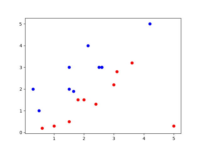
2.1 数据
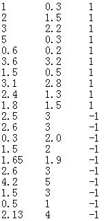
在二维坐标图中表示如下:
2.2 python实现
#!/usr/bin/python3
# -*- coding: utf-8 -*-
# @Time    : 2017/11/17 20:06
# @Author  : Z.C.Wang
# @Email   : iwangzhengchao@gmail.com
# @File    : PLA.py
# @Software: PyCharm Community Edition
"""
Description :
Perceptron learning algorithm
"""
import numpy as np
import matplotlib.pyplot as plt

# load data from txt
data_set = []
data_label = []
file = open('DataSet_linear_separable.txt')
for line in file:
    line = line.split('\t')
    for i in range(len(line)):
        line[i] = float(line[i])
    data_set.append(line[0:2])
    data_label.append(int(line[-1]))
file.close()
data = np.array(data_set)
label = np.array(data_label)
# 初始化w, b, alpha
w = np.array([0, 0])
b = 0
alpha = 1
# 计算 y*(w*x+b)
f = (np.dot(data, w.T) + b) * label
idx = np.where(f <= 0)
# 使用随机梯度下降法求解w, b
iteration = 1
while f[idx].size != 0:
    point = np.random.randint((f[idx].shape[0]))
    x = data[idx[0][point], :]
    y = label[idx[0][point]]
    w = w + alpha * y * x
    b = b + alpha * y
    print('Iteration:%d  w:%s  b:%s' % (iteration, w, b))
    f = (np.dot(data, w.T) + b) * label
    idx = np.where(f <= 0)
    iteration = iteration + 1

# 绘图显示
x1 = np.arange(0, 6, 0.1)
x2 = (w[0] * x1 + b) / (-w[1])
idx_p = np.where(label == 1)
idx_n = np.where(label != 1)
data_p = data[idx_p]
data_n = data[idx_n]
plt.scatter(data_p[:, 0], data_p[:, 1], color='red')
plt.scatter(data_n[:, 0], data_n[:, 1], color='blue')
plt.plot(x1, x2)
plt.show()
print('\nPerceptron learning algorithm is over')
#!/usr/bin/python3
# -*- coding: utf-8 -*-
# @Time : 2017/11/17 20:06
# @Author : Z.C.Wang
# @Email : iwangzhengchao@gmail.com
# @File : PLA.py
# @Software: PyCharm Community Edition
"""
Description :
Perceptron learning algorithm
"""
import numpy as np
import matplotlib.pyplot as plt
# load data from txt
data_set = []
data_label = []
file = open('DataSet_linear_separable.txt')
for line in file:
line = line.split('\t')
for i in range(len(line)):
line[i] = float(line[i])
data_set.append(line[0:2])
data_label.append(int(line[-1]))
file.close()
data = np.array(data_set)
label = np.array(data_label)
# 初始化w, b, alpha
w = np.array([0, 0])
b = 0
alpha = 1
# 计算 y*(w*x+b)
f = (np.dot(data, w.T) + b) * label
idx = np.where(f <= 0)
# 使用随机梯度下降法求解w, b
iteration = 1
while f[idx].size != 0:
point = np.random.randint((f[idx].shape[0]))
x = data[idx[0][point], :]
y = label[idx[0][point]]
w = w + alpha * y * x
b = b + alpha * y
print('Iteration:%d w:%s b:%s' % (iteration, w, b))
f = (np.dot(data, w.T) + b) * label
idx = np.where(f <= 0)
iteration = iteration + 1
# 绘图显示
x1 = np.arange(0, 6, 0.1)
x2 = (w[0] * x1 + b) / (-w[1])
idx_p = np.where(label == 1)
idx_n = np.where(label != 1)
data_p = data[idx_p]
data_n = data[idx_n]
plt.scatter(data_p[:, 0], data_p[:, 1], color='red')
plt.scatter(data_n[:, 0], data_n[:, 1], color='blue')
plt.plot(x1, x2)
plt.show()
print('\nPerceptron learning algorithm is over')
2.3 运行结果
结果如下:
Iteration:1  w:[-4.2 -5. ]  b:-1
Iteration:2  w:[-2.2 -3.5]  b:0
Iteration:3  w:[-0.2 -2. ]  b:1
Iteration:4  w:[ 2.2 -0.7]  b:2
Iteration:5  w:[-0.4 -3.7]  b:1
Iteration:6  w:[ 1.4 -2.2]  b:2
Iteration:7  w:[ 0.9 -3.2]  b:1
Iteration:8  w:[ 3.3 -1.9]  b:2
Iteration:9  w:[ 1.65 -3.8 ]  b:1
Iteration:10  w:[ 4.65 -1.6 ]  b:2
Iteration:11  w:[ 2.05 -4.6 ]  b:1
Iteration:12  w:[ 4.05 -3.1 ]  b:2
Iteration:13  w:[ 2.4 -5. ]  b:1
Iteration:14  w:[ 5.5 -2.2]  b:2
Iteration:15  w:[ 3.85 -4.1 ]  b:1

Perceptron learning algorithm is over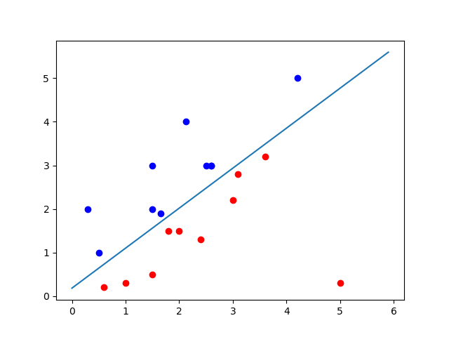


 1311
1311

 被折叠的 条评论
为什么被折叠?
被折叠的 条评论
为什么被折叠?
 到【灌水乐园】发言


