python gamma矫正

原文：http://blog.csdn.net/matrix_space/article/details/52415503

Python: scikit-image gamma and log 对比度调整

标签： python

2016-09-02 17:34  1453人阅读  评论(0)  收藏  举报

  分类：

图像处理（145） 

这个函数，主要用来做对比度调整，利用 gamma 曲线 或者 log 函数曲线，

gamma 函数的表达式： 
y=xγ , 其中，  x  是输入的像素值，取值范围为  [0−1] ,  y  是输出的像素值，通过调整 γ  值，改变图像的像素值的分布，进而改变图像的对比度。 
log 函数的表达式: 
y=alog(1+x) ,  a  是一个放大系数， x  同样是输入的像素值，取值范围为  [0−1] ,  y  是输出的像素值。 
inverse log 的表达式: 
y=a(2x−1) , 这些变换都是从  [0−1]  变到  [0−1]  。

"""
=================================
Gamma and log contrast adjustment
=================================

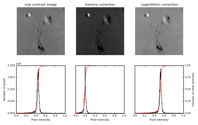
This example adjusts image contrast by performing a Gamma and a Logarithmic
correction on the input image.

"""
import matplotlib
import matplotlib.pyplot as plt
import numpy as np

from skimage import data, img_as_float
from skimage import exposure

matplotlib.rcParams['font.size'] = 8

def plot_img_and_hist(img, axes, bins=256):
    """Plot an image along with its histogram and cumulative histogram.
    """
    img = img_as_float(img)
    ax_img, ax_hist = axes
    ax_cdf = ax_hist.twinx()

    # Display image
    ax_img.imshow(img, cmap=plt.cm.gray)
    ax_img.set_axis_off()

    # Display histogram
    ax_hist.hist(img.ravel(), bins=bins, histtype='step', color='black')
    ax_hist.ticklabel_format(axis='y', style='scientific', scilimits=(0, 0))
    ax_hist.set_xlabel('Pixel intensity')
    ax_hist.set_xlim(0, 1)
    ax_hist.set_yticks([])

    # Display cumulative distribution
    img_cdf, bins = exposure.cumulative_distribution(img, bins)
    ax_cdf.plot(bins, img_cdf, 'r')
    ax_cdf.set_yticks([])

    return ax_img, ax_hist, ax_cdf


# Load an example image
img = data.moon()

# Gamma
gamma_corrected = exposure.adjust_gamma(img, 2)

# Logarithmic
logarithmic_corrected = exposure.adjust_log(img, 1)

# Display results
fig = plt.figure(figsize=(8, 5))
axes = np.zeros((2, 3), dtype=np.object)
axes[0, 0] = plt.subplot(2, 3, 1, adjustable='box-forced')

axes[0, 1] = plt.subplot(2, 3, 2, sharex=axes[0, 0], sharey=axes[0, 0],
                         adjustable='box-forced')

axes[0, 2] = plt.subplot(2, 3, 3, sharex=axes[0, 0], sharey=axes[0, 0],
                         adjustable='box-forced')

axes[1, 0] = plt.subplot(2, 3, 4)
axes[1, 1] = plt.subplot(2, 3, 5)
axes[1, 2] = plt.subplot(2, 3, 6)

ax_img, ax_hist, ax_cdf = plot_img_and_hist(img, axes[:, 0])
ax_img.set_title('Low contrast image')

y_min, y_max = ax_hist.get_ylim()
ax_hist.set_ylabel('Number of pixels')
ax_hist.set_yticks(np.linspace(0, y_max, 5))

ax_img, ax_hist, ax_cdf = plot_img_and_hist(gamma_corrected, axes[:, 1])
ax_img.set_title('Gamma correction')

ax_img, ax_hist, ax_cdf = plot_img_and_hist(logarithmic_corrected, axes[:, 2])
ax_img.set_title('Logarithmic correction')

ax_cdf.set_ylabel('Fraction of total intensity')
ax_cdf.set_yticks(np.linspace(0, 1, 5))

# prevent overlap of y-axis labels
fig.tight_layout()
plt.show()

   
   
1
2
3
4
5
6
7
8
9
10
11
12
13
14
15
16
17
18
19
20
21
22
23
24
25
26
27
28
29
30
31
32
33
34
35
36
37
38
39
40
41
42
43
44
45
46
47
48
49
50
51
52
53
54
55
56
57
58
59
60
61
62
63
64
65
66
67
68
69
70
71
72
73
74
75
76
77
78
79
80
81
82
83
84
85
86
87
88