


学习Python中的一些数学函数与函数的绘图
主要用到numpy 与 matplotlib
如果有什么不正确,欢迎指教。
图片不知道怎样批量上传,一个一个怎么感觉很小,请见谅
自行复制拷贝,到vs,jupyter notebook, spyder都可以
函数 y = x − s i n x y = x - sinx y=x−sinx
%matplotlib inline
%config InlineBackend.figure_format = "svg"
import numpy as np
import matplotlib.pyplot as plt
from scipy import signal
plt.rcParams['figure.figsize'] = (8, 4.5)
plt.rcParams['figure.dpi'] = 150
plt.rcParams['font.sans-serif'] = ['Simhei']  #替代字体
plt.rcParams['axes.unicode_minus'] = False  #解决坐标轴负数的铅显示问题

x1 = np.linspace(-np.pi, np.pi, 1000)
y1 = x1 - np.sin(x1)

plt.plot(x1, y1, c = 'k', label = r"$ y=x-sinx $")

plt.grid()
plt.legend()
plt.show()

函数 y = 3 x 4 − 4 x 3 + 1 y = 3x^4 - 4x^3 + 1 y=3x4−4x3+1
%matplotlib inline
%config InlineBackend.figure_format = "svg"
import numpy as np
import matplotlib.pyplot as plt
from scipy import signal
plt.rcParams['figure.figsize'] = (8, 4.5)
plt.rcParams['figure.dpi'] = 150
plt.rcParams['font.sans-serif'] = ['Simhei']  #替代字体
plt.rcParams['axes.unicode_minus'] = False  #解决坐标轴负数的铅显示问题

x1 = np.linspace(-1, 1.5, 1000)
y1 = 3 * (x1 ** 4) - 4 * (x1 ** 3) + 1
plt.plot(x1, y1, label = r"$ y = 3x^4 - 4x^3 + 1 $")

plt.grid()
plt.legend()
plt.show()

函数 y = x 4 y = x^4 y=x4
%matplotlib inline
%config InlineBackend.figure_format = "svg"
import numpy as np
import matplotlib.pyplot as plt
from scipy import signal
plt.rcParams['figure.figsize'] = (8, 4.5)
plt.rcParams['figure.dpi'] = 150
plt.rcParams['font.sans-serif'] = ['Simhei']  #替代字体
plt.rcParams['axes.unicode_minus'] = False  #解决坐标轴负数的铅显示问题

x1 = np.linspace(-5, 5, 1000)
y1 = x1 ** 4

plt.plot(x1, y1, label = r"$ y = x^4 $")

plt.grid()
plt.legend()
plt.show()

函数 y = x 3 y = \sqrt[3]{x} y=3x
%matplotlib inline
%config InlineBackend.figure_format = "svg"
import numpy as np
import matplotlib.pyplot as plt
from scipy import signal
plt.rcParams['figure.figsize'] = (8, 4.5)
plt.rcParams['figure.dpi'] = 150
plt.rcParams['font.sans-serif'] = ['Simhei']  #替代字体
plt.rcParams['axes.unicode_minus'] = False  #解决坐标轴负数的铅显示问题

x1 = np.linspace(0, 5, 1000)
y1 = x1 ** (1/3)

plt.plot(x1, y1, label = r"$ y = \sqrt[3]{x} $")


# plt.xlim([-np.pi, np.pi])
# plt.ylim([-1.5, 1.5])
plt.grid()
plt.legend()
plt.show()

函数 y = 2 x 3 − 9 x 2 + 12 x − 3 y=2x^3-9x^2+12x-3 y=2x3−9x2+12x−3
%matplotlib inline
%config InlineBackend.figure_format = "svg"
import numpy as np
import matplotlib.pyplot as plt
from scipy import signal
plt.rcParams['figure.figsize'] = (8, 4.5)
plt.rcParams['figure.dpi'] = 150
plt.rcParams['font.sans-serif'] = ['Simhei']  #替代字体
plt.rcParams['axes.unicode_minus'] = False  #解决坐标轴负数的铅显示问题

x1 = np.linspace(-2, 5, 1000)
y1 =2 * (x1 ** 3) - 9 * (x1 ** 2) + 12 * x1 - 3

plt.plot(x1, y1, label = r"$ y=2x^3-9x^2+12x-3 $")

plt.grid()
plt.legend()
plt.show()

函数 y = 2 x 3 − 6 x 2 − 18 x + 7 y=2x^3-6x^2-18x+7 y=2x3−6x2−18x+7
%matplotlib inline
%config InlineBackend.figure_format = "svg"
import numpy as np
import matplotlib.pyplot as plt
from scipy import signal
plt.rcParams['figure.figsize'] = (8, 4.5)
plt.rcParams['figure.dpi'] = 150
plt.rcParams['font.sans-serif'] = ['Simhei']  #替代字体
plt.rcParams['axes.unicode_minus'] = False  #解决坐标轴负数的铅显示问题

x1 = np.linspace(-3, 5, 1000)
y1 = 2 * (x1 ** 3) - 6 * (x1 ** 2) - 18 * x1 + 7

plt.plot(x1, y1, label = r"$ y=2x^3-6x^2-18x+7 $")

# plt.axis('equal')
plt.grid()
plt.legend()
plt.show()

三次抛物线 y = x 3 y = x^3 y=x3
%matplotlib inline
%config InlineBackend.figure_format = "svg"
import numpy as np
import matplotlib.pyplot as plt
from scipy import signal
plt.rcParams['figure.figsize'] = (8, 4.5)
plt.rcParams['figure.dpi'] = 150
plt.rcParams['font.sans-serif'] = ['Simhei']  #替代字体
plt.rcParams['axes.unicode_minus'] = False  #解决坐标轴负数的铅显示问题

ax = plt.gca()
ax.spines['right'].set_color('none')
ax.spines['top'].set_color('none')
ax.xaxis.set_ticks_position('bottom')
ax.spines['bottom'].set_position(('data', 0))
ax.yaxis.set_ticks_position('left')
ax.spines['left'].set_position(('data', 0))

x1 = np.linspace(-5, 5, 1000)
y1 = x1 ** 3

plt.plot(x1, y1, label = r"$ y = x^3 $")

plt.grid()
plt.legend()
plt.show()

半立方抛物线 y 2 = a x 3 y^2 = ax^3 y2=ax3
%matplotlib inline
%config InlineBackend.figure_format = "svg"
import numpy as np
import matplotlib.pyplot as plt
from scipy import signal
plt.rcParams['figure.figsize'] = (8, 4.5)
plt.rcParams['figure.dpi'] = 150
plt.rcParams['font.sans-serif'] = ['Simhei']  #替代字体
plt.rcParams['axes.unicode_minus'] = False  #解决坐标轴负数的铅显示问题

a = 0.1
t = np.linspace(-5, 5, 1000)
x = t ** 2
y = a * (t ** 3)
plt.plot(x, y, label = r"y^2 = ax^3|a=0.1")

a = 1
y1 = a * (t ** 3)
plt.plot(x, y1, label = r"y^2 = ax^3|a=1")


# plt.xlim([-np.pi, np.pi])
# plt.ylim([-1.5, 1.5])
plt.grid()
plt.legend()
plt.show()

概率曲线 y = e − x 2 y=e^{-x^2} y=e−x2
%matplotlib inline
%config InlineBackend.figure_format = "svg"
import numpy as np
import matplotlib.pyplot as plt
from scipy import signal
plt.rcParams['figure.figsize'] = (8, 4.5)
plt.rcParams['figure.dpi'] = 150
plt.rcParams['font.sans-serif'] = ['Simhei']  #替代字体
plt.rcParams['axes.unicode_minus'] = False  #解决坐标轴负数的铅显示问题

t = np.linspace(-2, 2, 1000)
x = t
y = np.e ** -(x ** 2)
plt.plot(x, y, label = r"$ y=e^{-x^2} $")

plt.axis('equal')
# plt.grid()
plt.legend()
plt.show()

箕舌线 y = 8 a 3 x 2 + 4 a 2 y =\frac{8a^3}{x^2+4a^2} y=x2+4a28a3
%matplotlib inline
%config InlineBackend.figure_format = "svg"
import numpy as np
import matplotlib.pyplot as plt
from scipy import signal
plt.rcParams['figure.figsize'] = (8, 4.5)
plt.rcParams['figure.dpi'] = 150
plt.rcParams['font.sans-serif'] = ['Simhei']  #替代字体
plt.rcParams['axes.unicode_minus'] = False  #解决坐标轴负数的铅显示问题

a = 1
t = np.linspace(-5, 5, 1000)
x = t
y = (8 * a ** 2) / (x ** 2 + 4 * a ** 2)
plt.plot(x, y, label = r"$ y =\frac{8a^3}{x^2+4a^2} |_{a=1} $")

a = 2
y1 = (8 * a ** 2) / (x ** 2 + 4 * a ** 2)
plt.plot(x, y1, label = r"$ y =\frac{8a^3}{x^2+4a^2} |_{a=2} $")

plt.axis('equal')
# plt.grid()
plt.legend()
plt.show()

蔓叶线 y 2 ( 2 a − x ) = x 3 y^2(2a-x)=x^3 y2(2a−x)=x3 或 x = 2 a s i n 2 θ , y = 2 a 2 t a n 2 θ s i n 4 θ x=2asin^2\theta, y=2a^2tan^2\theta sin^4\theta x=2asin2θ,y=2a2tan2θsin4θ
修改:之前x的取值是 − 3.6 ≤ x ≤ 3.6 -3.6\leq x \leq3.6 −3.6≤x≤3.6, 实际上x的值是 ≥ 0 \geq 0 ≥0
%matplotlib inline
%config InlineBackend.figure_format = "svg"
import numpy as np
import matplotlib.pyplot as plt
from scipy import signal
plt.rcParams['figure.figsize'] = (8, 4.5)
plt.rcParams['figure.dpi'] = 150
plt.rcParams['font.sans-serif'] = ['Simhei']  #替代字体
plt.rcParams['axes.unicode_minus'] = False  #解决坐标轴负数的铅显示问题

a = 2
#这是原来的取值范围
#t = np.linspace(-3.6, 3.6, 1000)
#x = np.abs(t)
#这是现在的取值范围
t = np.linspace(0, 3.6, 1000)
x = t
#还有我用power替代了sqrt开根号
y = np.power((x ** 3) / (2 * a - x), 1/2)
plt.plot(x, y, 'b', x, -y, 'b', label = r"$ y^2(2a-x)=x^3 $")

plt.grid()
plt.legend()
plt.show()

ρ = 2 a − t a n 2 θ \rho=2a-tan^2\theta ρ=2a−tan2θ
%matplotlib inline
%config InlineBackend.figure_format = "svg"
import numpy as np
import matplotlib.pyplot as plt
from scipy import signal
plt.rcParams['figure.figsize'] = (8, 4.5)
plt.rcParams['figure.dpi'] = 150
plt.rcParams['font.sans-serif'] = ['Simhei']  #替代字体
plt.rcParams['axes.unicode_minus'] = False  #解决坐标轴负数的铅显示问题

#极坐标
plt.subplot(111, polar = True)
plt.ylim([0, 6])

a = 1
theta = np.arange(0, 2 * np.pi, np.pi / 100)
rho = 2 * a - np.tan(theta) ** 2
plt.plot(theta, rho, label = r'$\rho=2a-tan^2\theta \quad |a=1$')

a = 1.5
r2 = a * rho
plt.plot(theta, r2, label = r'$\rho=2a-tan^2\theta \quad |a=1.5$')

a = 2.5
r2 = a * rho
plt.plot(theta, r2, label = r'$\rho=2a-tan^2\theta \quad |a=2.5$')

plt.legend()
plt.show()

笛卡儿叶形线画图 极坐标 r = 3 a s i n θ c o s θ s i n 3 θ + c o s 3 θ r = \frac{3asin\theta cos\theta}{sin^3\theta + cos^3\theta} r=sin3θ+cos3θ3asinθcosθ
%matplotlib inline
%config InlineBackend.figure_format = "svg"
import numpy as np
import matplotlib.pyplot as plt
from scipy import signal
plt.rcParams['figure.figsize'] = (8, 4.5)
plt.rcParams['figure.dpi'] = 150
plt.rcParams['font.sans-serif'] = ['Simhei']  #替代字体
plt.rcParams['axes.unicode_minus'] = False  #解决坐标轴负数的铅显示问题

#极坐标
plt.subplot(111, polar = True)
plt.ylim([0, 6])

a = 1
theta = np.arange(0, 2 * np.pi, np.pi / 100)
r = 3 * a * np.sin(theta) * np.cos(theta) / (np.sin(theta) ** 3 + np.cos(theta) ** 3)
plt.plot(theta, r, label = r'$ r = \frac{3asin\theta cos\theta}{sin^3\theta + cos^3\theta} $')

a = 1.5
r2 = a * r
plt.plot(theta, r2)

a = 2.5
r2 = a * r
plt.plot(theta, r2)

# plt.grid()
plt.legend()
plt.show()

笛卡儿叶形线 直角坐标 x 3 + y 3 − 3 a x y = 0 x^3+y^3-3axy=0 x3+y3−3axy=0 或 x = 3 a t 1 + t 3 , y = 3 a t 2 1 + t 3 x=\frac{3at}{1+t^3}, y=\frac{3at^2}{1+t^3} x=1+t33at,y=1+t33at2
%matplotlib inline
%config InlineBackend.figure_format = "svg"
import numpy as np
import matplotlib.pyplot as plt
from scipy import signal
plt.rcParams['figure.figsize'] = (8, 4.5)
plt.rcParams['figure.dpi'] = 150
plt.rcParams['font.sans-serif'] = ['Simhei']  #替代字体
plt.rcParams['axes.unicode_minus'] = False  #解决坐标轴负数的铅显示问题

#极坐标
# plt.subplot(111, polar = True)
# plt.ylim([0, 6])

a = 1
# t = np.arange(-0.1, 4 * np.pi, np.pi / 180)
t = np.linspace(-0.5, 200, 5000)
x = (3 * a * t) / (1 + t ** 3)
y = (3 * a * t ** 2) / (1 + t ** 3)
plt.plot(x, y, label = r'$ x=\frac{3at}{1+t^3}, y=\frac{3at^2}{1+t^3} $')

a = 1.5
x1 = (3 * a * t) / (1 + t ** 3)
y1 = (3 * a * t ** 2) / (1 + t ** 3)
plt.plot(x1, y1, label = r'$ x=\frac{3at}{1+t^3}, y=\frac{3at^2}{1+t^3} $')


# plt.grid()
plt.legend()
plt.show()

星形线(内摆线的一种) x 2 3 + y 2 3 = a 2 3 x^\frac{2}{3}+y^\frac{2}{3}=a^\frac{2}{3} x32+y32=a32 或 { x = a c o s 3 θ y = a s i n 3 θ \begin{cases} x=acos^3\theta \\ y=asin^3\theta \end{cases} {x=acos3θy=asin3θ
%matplotlib inline
%config InlineBackend.figure_format = "svg"
import numpy as np
import matplotlib.pyplot as plt
from scipy import signal
plt.rcParams['figure.figsize'] = (8, 4.5)
plt.rcParams['figure.dpi'] = 150
plt.rcParams['font.sans-serif'] = ['Simhei']  #替代字体
plt.rcParams['axes.unicode_minus'] = False  #解决坐标轴负数的铅显示问题

a = 1
theta = np.arange(0, 2 * np.pi, np.pi / 180)
x = a * np.cos(theta) ** 3
y = a * np.sin(theta) ** 3
plt.plot(x, y, label = r'$ x=acos^3\theta, y=asin^3\theta \quad|a=1$')

a = 2
x1 = a * x
y1 = a * y
plt.plot(x1, y1, label = r'$ x=acos^3\theta, y=asin^3\theta \quad|a=2$')

a = 3
x2 = a * x
y2 = a * y
plt.plot(x2, y2, label = r'$ x=acos^3\theta, y=asin^3\theta \quad|a=3$')

ax = plt.gca()
ax.spines['right'].set_color('none')
ax.spines['top'].set_color('none')
ax.xaxis.set_ticks_position('bottom')
ax.spines['bottom'].set_position(('data', 0))
ax.yaxis.set_ticks_position('left')
ax.spines['left'].set_position(('data', 0))


plt.axis('equal')
plt.legend()
plt.show()

摆线 { x = a ( θ − s i n θ ) y = a ( 1 − c o s θ ) \begin{cases} x=a(\theta-sin\theta) \\ y=a(1-cos\theta) \end{cases} {x=a(θ−sinθ)y=a(1−cosθ)
%matplotlib inline
%config InlineBackend.figure_format = "svg"
import numpy as np
import matplotlib.pyplot as plt
from scipy import signal
plt.rcParams['figure.figsize'] = (8, 4.5)
plt.rcParams['figure.dpi'] = 150
plt.rcParams['font.sans-serif'] = ['Simhei']  #替代字体
plt.rcParams['axes.unicode_minus'] = False  #解决坐标轴负数的铅显示问题

#极坐标
# plt.subplot(111, polar = True)
# plt.ylim([0, 6])

a = 1
theta = np.arange(0, 4 * np.pi, np.pi / 180)
x = a * (theta - np.sin(theta))
y = a * (1 - np.cos(theta))
plt.plot(x, y, label = r'$ x=a(\theta-sin\theta),\quad y=a(1-cos\theta) \quad|a=1$')

a = 2
x1 = a * x
y1 = a * y
plt.plot(x1, y1, label = r'$ x=a(\theta-sin\theta),\quad y=a(1-cos\theta) \quad|a=2$')

a = 3
x2 = a * x
y2 = a * y
plt.plot(x2, y2, label = r'$ x=a(\theta-sin\theta),\quad y=a(1-cos\theta) \quad|a=3$')

ax = plt.gca()
ax.spines['right'].set_color('none')
ax.spines['top'].set_color('none')
ax.xaxis.set_ticks_position('bottom')
ax.spines['bottom'].set_position(('data', 0))
ax.yaxis.set_ticks_position('left')
ax.spines['left'].set_position(('data', 0))


plt.axis('equal')
plt.legend()
plt.show()

心形线(外摆线的一种) KaTeX parse error: Can't use function '$' in math mode at position 27: …a\sqrt{x^2+y^2}$̲ 或 $ \rho=a(1-c…
%matplotlib inline
%config InlineBackend.figure_format = "svg"
import numpy as np
import matplotlib.pyplot as plt
from scipy import signal
plt.rcParams['figure.figsize'] = (8, 4.5)
plt.rcParams['figure.dpi'] = 150
plt.rcParams['font.sans-serif'] = ['Simhei']  #替代字体
plt.rcParams['axes.unicode_minus'] = False  #解决坐标轴负数的铅显示问题

#极坐标
plt.subplot(111, polar = True)
# plt.ylim([0, 6])

a = 1
theta = np.arange(0, 2 * np.pi, np.pi / 180)
y = a * (1 - np.cos(theta))
plt.plot(theta, y, label = r'$ \rho=a(1-cos\theta) $')

y1 = a * (1 - np.sin(theta))
plt.plot(theta, y1, label = r'$ \rho=a(1-sin\theta) $')

# a = 2
# x1 = a * x
# y1 = a * y
# plt.plot(x1, y1, label = r'$ x=a(\theta-sin\theta),\quad y=a(1-cos\theta) \quad|a=2$')

# a = 3
# x2 = a * x
# y2 = a * y
# plt.plot(x2, y2, label = r'$ x=a(\theta-sin\theta),\quad y=a(1-cos\theta) \quad|a=3$')

# ax = plt.gca()
# ax.spines['right'].set_color('none')
# ax.spines['top'].set_color('none')
# ax.xaxis.set_ticks_position('bottom')
# ax.spines['bottom'].set_position(('data', 0))
# ax.yaxis.set_ticks_position('left')
# ax.spines['left'].set_position(('data', 0))


# plt.axis('equal')
plt.legend()
plt.show()

x = s i n θ , y = c o s θ + x 2 3 x=sin\theta,\quad y=cos\theta+\sqrt[3]{x^2} x=sinθ,y=cosθ+3x2
%matplotlib inline
%config InlineBackend.figure_format = "svg"
import numpy as np
import matplotlib.pyplot as plt
from scipy import signal
plt.rcParams['figure.figsize'] = (8, 4.5)
plt.rcParams['figure.dpi'] = 150
plt.rcParams['font.sans-serif'] = ['Simhei']  #替代字体
plt.rcParams['axes.unicode_minus'] = False  #解决坐标轴负数的铅显示问题


a = 1
theta = np.arange(0, 2 * np.pi, np.pi / 180)
x = np.sin(theta)
y = np.cos(theta) + np.power((x ** 2), 1 / 3)  #原来用 y = np.cos(theta) + np.power(x, 2/3)只画出一半,而且报power的错
plt.plot(x, y, label = r'$x=sin\theta,\quady=cos\theta+\sqrt[3]{x^2}$')


# ax = plt.gca()
# ax.spines['right'].set_color('none')
# ax.spines['top'].set_color('none')
# ax.xaxis.set_ticks_position('bottom')
# ax.spines['bottom'].set_position(('data', 0))
# ax.yaxis.set_ticks_position('left')
# ax.spines['left'].set_position(('data', 0))


plt.axis('equal') #等比例会好看点
plt.legend()
plt.show()

阿基米德螺线 ρ = a θ \rho=a\theta ρ=aθ
%matplotlib inline
%config InlineBackend.figure_format = "svg"
import numpy as np
import matplotlib.pyplot as plt
from scipy import signal
plt.rcParams['figure.figsize'] = (8, 4.5)
plt.rcParams['figure.dpi'] = 150
plt.rcParams['font.sans-serif'] = ['Simhei']  #替代字体
plt.rcParams['axes.unicode_minus'] = False  #解决坐标轴负数的铅显示问题

#极坐标
plt.subplot(111, polar = True)
# plt.ylim([0, 6])

a = 1
theta = np.arange(0, 4 * np.pi, np.pi / 180)
rho = a * theta
plt.plot(theta, rho, label = r'$\rho=a\theta$', linestyle = 'solid')

# rho1 = - a * theta
# plt.plot(theta, rho1, label = r'$\rho=a\theta$')


plt.legend()
plt.show()

对数螺线 ρ = e a θ \rho=e^{a\theta} ρ=eaθ
%matplotlib inline
%config InlineBackend.figure_format = "svg"
import numpy as np
import matplotlib.pyplot as plt
from scipy import signal
plt.rcParams['figure.figsize'] = (8, 4.5)
plt.rcParams['figure.dpi'] = 150
plt.rcParams['font.sans-serif'] = ['Simhei']  #替代字体
plt.rcParams['axes.unicode_minus'] = False  #解决坐标轴负数的铅显示问题

#极坐标
plt.subplot(111, polar = True)
plt.ylim([0, 10])

a = 0.1
theta = np.arange(0, 6 * np.pi, np.pi / 180)
rho = np.e ** (a * theta)
plt.plot(theta, rho, label = r'$ \rho=e^{a\theta} $', linestyle = 'solid')

a = 0.2
rho1 = np.e ** (a * theta)
plt.plot(theta, rho1, label = r'$ \rho=e^{a\theta} $', linestyle = 'solid')

plt.legend()
plt.show()

双曲螺旋线 ρ θ = a \rho\theta=a ρθ=a
%matplotlib inline
%config InlineBackend.figure_format = "svg"
import numpy as np
import matplotlib.pyplot as plt
from scipy import signal
plt.rcParams['figure.figsize'] = (8, 4.5)
plt.rcParams['figure.dpi'] = 150
plt.rcParams['font.sans-serif'] = ['Simhei']  #替代字体
plt.rcParams['axes.unicode_minus'] = False  #解决坐标轴负数的铅显示问题

#极坐标
plt.subplot(111, polar = True)
plt.ylim([0, 30])

a = 30
theta = np.arange(0.01, 6 * np.pi, np.pi / 180)
rho = a / theta
plt.plot(theta, rho, label = r'$ \rho\theta=a \quad |a=30 $', linestyle = 'solid')

a = 50
rho1 = a / theta
plt.plot(theta, rho1, label = r'$ \rho\theta=a \quad |a=50 $', linestyle = 'solid')

plt.legend()
plt.show()

伯努利双纽线 ( x 2 + y 2 ) 2 = 2 a 2 x y (x^2+y^2)^2=2a^2xy (x2+y2)2=2a2xy 或 ( x 2 + y 2 ) 2 = a 2 ( x 2 − y 2 ) (x^2+y^2)^2=a^2(x^2-y^2) (x2+y2)2=a2(x2−y2) 或 ρ 2 = a 2 s i n 2 θ \rho^2=a^2sin2\theta ρ2=a2sin2θ 或 ρ 2 = a 2 c o s 2 θ \rho^2=a^2cos2\theta ρ2=a2cos2θ
%matplotlib inline
%config InlineBackend.figure_format = "svg"
import numpy as np
import matplotlib.pyplot as plt
from scipy import signal
plt.rcParams['figure.figsize'] = (8, 4.5)
plt.rcParams['figure.dpi'] = 150
plt.rcParams['font.sans-serif'] = ['Simhei']  #替代字体
plt.rcParams['axes.unicode_minus'] = False  #解决坐标轴负数的铅显示问题

#极坐标
# plt.subplot(111, polar = True)
# plt.ylim([0, 30])

a = 1
theta = np.linspace(-np.pi, np.pi, 200)
x = a * np.sqrt(2) * np.cos(theta) / (np.sin(theta) ** 2 + 1)
y = a * np.sqrt(2) * np.cos(theta) * np.sin(theta) / (np.sin(theta) ** 2 + 1)
plt.plot(x, y, label = r'$ \rho^2=a^2cos2\theta \quad |a=1 $', linestyle = 'solid')

plt.axis('equal')
plt.legend()
plt.show()

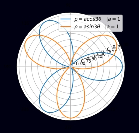
三叶玫瑰线 ρ = a c o s 3 θ \rho=acos3\theta ρ=acos3θ 或 ρ = a s i n 3 θ \rho=asin3\theta ρ=asin3θ
%matplotlib inline
%config InlineBackend.figure_format = "svg"
import numpy as np
import matplotlib.pyplot as plt
from scipy import signal
# plt.rcParams['figure.figsize'] = (8, 4.5)
# plt.rcParams['figure.dpi'] = 150
plt.rcParams['font.sans-serif'] = ['Simhei']  #替代字体
plt.rcParams['axes.unicode_minus'] = False  #解决坐标轴负数的铅显示问题

#极坐标
plt.subplot(111, polar = True)
# plt.ylim([0, 30])

a = 1
theta = np.linspace(0, 2 * np.pi, 200)
rho = a * np.cos(3 * theta)
plt.plot(theta, rho, label = r'$ \rho=acos3\theta \quad |a=1 $', linestyle = 'solid')

# a = 2
# rho1 = a * rho
# plt.plot(theta, rho1, label = r'$ \rho=acos3\theta \quad |a=2 $', linestyle = 'solid')

a = 1
rho2 = a * np.sin(3 * theta)
plt.plot(theta, rho2, label = r'$ \rho=asin3\theta \quad |a=1 $', linestyle = 'solid')

plt.legend()
plt.show()
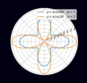
四叶玫瑰线 ρ = a c o s 2 θ \rho=acos2\theta ρ=acos2θ 或 ρ = a s i n 2 θ \rho=asin2\theta ρ=asin2θ
%matplotlib inline
%config InlineBackend.figure_format = "svg"
import numpy as np
import matplotlib.pyplot as plt
from scipy import signal
# plt.rcParams['figure.figsize'] = (8, 4.5)
# plt.rcParams['figure.dpi'] = 150
plt.rcParams['font.sans-serif'] = ['Simhei']  #替代字体
plt.rcParams['axes.unicode_minus'] = False  #解决坐标轴负数的铅显示问题

#极坐标
plt.subplot(111, polar = True)
# plt.ylim([0, 30])

a = 1
theta = np.linspace(0, 2 * np.pi, 200)
rho = a * np.cos(4 * theta)
plt.plot(theta, rho, label = r'$ \rho=acos2\theta \quad |a=1 $', linestyle = 'solid')

a = 2
rho1 = a * rho
plt.plot(theta, rho1, label = r'$ \rho=acos2\theta \quad |a=2 $', linestyle = 'solid')

# a = 1
# rho2 = a * np.sin(4 * theta)
# plt.plot(theta, rho2, label = r'$ \rho=asin2\theta \quad |a=1 $', linestyle = 'solid')

plt.legend()
plt.show()
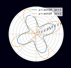
%matplotlib inline
%config InlineBackend.figure_format = "svg"
import numpy as np
import matplotlib.pyplot as plt
from scipy import signal
# plt.rcParams['figure.figsize'] = (8, 4.5)
# plt.rcParams['figure.dpi'] = 150
plt.rcParams['font.sans-serif'] = ['Simhei']  #替代字体
plt.rcParams['axes.unicode_minus'] = False  #解决坐标轴负数的铅显示问题

#极坐标
plt.subplot(111, polar = True)
# plt.ylim([0, 30])

theta = np.linspace(0, 2 * np.pi, 200)

a = 1
rho = a * np.sin(4 * theta)
plt.plot(theta, rho, label = r'$ \rho=asin2\theta \quad |a=1 $', linestyle = 'solid')

a = 2
rho1 = a * np.sin(4 * theta)
plt.plot(theta, rho1, label = r'$ \rho=asin2\theta \quad |a=2 $', linestyle = '--')

plt.legend()
plt.show()
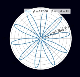
多叶玫瑰线 ρ = a c o s n θ \rho=acosn\theta ρ=acosnθ 或 ρ = a s i n n θ , ∣ n = 1 , 2 , 3... \rho=asinn\theta,\quad|n=1,2,3... ρ=asinnθ,∣n=1,2,3...
%matplotlib inline
%config InlineBackend.figure_format = "svg"
import numpy as np
import matplotlib.pyplot as plt
from scipy import signal
# plt.rcParams['figure.figsize'] = (8, 4.5)
# plt.rcParams['figure.dpi'] = 150
plt.rcParams['font.sans-serif'] = ['Simhei']  #替代字体
plt.rcParams['axes.unicode_minus'] = False  #解决坐标轴负数的铅显示问题

#极坐标
plt.subplot(111, polar = True)
# plt.ylim([0, 30])

theta = np.linspace(0, 2 * np.pi, 200)

a = 1
n = 20
rho = a * np.sin(10 * theta)
plt.plot(theta, rho, label = r'$ \rho=asinn\theta \quad |a=1,n=10 $', linestyle = 'solid')

plt.legend()
plt.show()
函数 四叶线 x = a ρ s i n θ , y = a ρ c o s θ , ρ = 2 s i n s i n 2 θ x=a\rho sin\theta,y=a\rho cos\theta, \rho = \sqrt{2}sin{sin2\theta} x=aρsinθ,y=aρcosθ,ρ=2sinsin2θ
%matplotlib inline
%config InlineBackend.figure_format = "svg"
import numpy as np
import matplotlib.pyplot as plt
from scipy import signal
plt.rcParams['figure.figsize'] = (8, 4.5)
plt.rcParams['figure.dpi'] = 150
plt.rcParams['font.sans-serif'] = ['Simhei']  #替代字体
plt.rcParams['axes.unicode_minus'] = False  #解决坐标轴负数的铅显示问题

#极坐标
# plt.subplot(111, polar = True)
# plt.ylim([0, 30])

a = 1
theta = np.linspace(-np.pi, np.pi, 200)
rho = np.sqrt(2) * np.sin(np.sin(2*theta))
x = a * rho * np.sin(theta)
y = a * rho * np.cos(theta)
plt.plot(x, y, label = r'$x=a\rho sin\theta,y=a\rho cos\theta, \rho = \sqrt{2}sin{sin2\theta}$', linestyle = 'solid')

plt.axis('equal')
plt.legend()
plt.show()
[外链图片转存失败,源站可能有防盗链机制,建议将图片保存下来直接上传(img-vELrwNwd-1589013522141)(output_52_0.svg)]
%matplotlib inline
%config InlineBackend.figure_format = "svg"
import numpy as np
import matplotlib.pyplot as plt
from scipy import signal
plt.rcParams['figure.figsize'] = (8, 4.5)
plt.rcParams['figure.dpi'] = 150
plt.rcParams['font.sans-serif'] = ['Simhei']  #替代字体
plt.rcParams['axes.unicode_minus'] = False  #解决坐标轴负数的铅显示问题

#极坐标
# plt.subplot(111, polar = True)
# plt.ylim([0, 30])

a = 1
theta = np.linspace(-np.pi, np.pi, 200)
rho = np.sqrt(2) * np.sin(np.sin(4*theta))
x = a * rho * np.sin(theta)
y = a * rho * np.cos(theta)
plt.plot(x, y, label = r'$x=a\rho sin\theta,y=a\rho cos\theta, \rho = \sqrt{2}sin{sin2\theta}$', linestyle = 'solid')

plt.axis('equal')
plt.legend()
plt.show()

函数 四叶线 x = a ρ s i n θ , y = a ρ c o s θ , ρ = 2 s i n ∣ s i n 2 θ ∣ x=a\rho sin\theta,y=a\rho cos\theta, \rho = \sqrt{2}sin{\vert sin2\theta \vert} x=aρsinθ,y=aρcosθ,ρ=2sin∣sin2θ∣
%matplotlib inline
%config InlineBackend.figure_format = "svg"
import numpy as np
import matplotlib.pyplot as plt
from scipy import signal
# plt.rcParams['figure.figsize'] = (8, 4.5)
# plt.rcParams['figure.dpi'] = 150
plt.rcParams['font.sans-serif'] = ['Simhei']  #替代字体
plt.rcParams['axes.unicode_minus'] = False  #解决坐标轴负数的铅显示问题

#极坐标
# plt.subplot(111, polar = True)
# plt.ylim([0, 30])

a = 1
theta = np.linspace(-np.pi, np.pi, 1000)
rho = np.sqrt(2) * np.sqrt(abs(np.sin(10*theta)) + 0.5)
x = a * rho * np.sin(theta)
y = a * rho * np.cos(theta)
plt.plot(x, y,  linestyle = 'solid')

# label = r'$x=a\rho sin\theta,y=a\rho cos\theta, \rho = \sqrt{2}sin{sin2\theta}$',

plt.axis('equal')
# plt.legend()
plt.show()


 1466
1466


 被折叠的 条评论
为什么被折叠?
被折叠的 条评论
为什么被折叠?
 到【灌水乐园】发言


