


目录
引言
旨在寻找图像间的对应点和对应区域,通过利用局部特征来现实创建全景图、增强现实技术、计算图像的三维重建。
一、Harris角点检测器
Harris角点检测算法是一种极其简单的角点检测算法,其主要思想为:当像素周围显示存在多于一个方向的边,就称该点为兴趣点(角点)。
将图像域中点x上的对称半正定矩阵定义为:
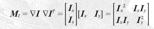
这其中中包含导数
的图像梯度,由于
的秩为1,特征值就为
以及
,根据这些信息,对于图像中的每一个像素,都可以计算出这个矩阵。
选择权重矩阵W(一般情况下为高斯滤波器),可以得到卷积:
![]()
其目的是得到在周围像素上的局部平均。计算得出的
又被称为Harris矩阵。矩阵W的宽度决定了像素x周围的感兴趣区域。在区域附近对矩阵
取平均的原因是,矩阵的特征值会依赖于局部图像特性而变化。若图像梯度在区域内发生变化,则Harris矩阵的第二个特征值就不再是0了,反之如果不发生变化,特征值也不变。
针对Harris矩阵的特征值一共有三种情况:
1、若都是很大的正数,该x点就是角点。
2、若很大,
,则区域内存在一个边,且平均
的特征值不会变化太大。
3、,区域为空。
Harris角点检测实验
在程序中我们还是要使用到scipy.ndimage.filters模块中的高斯导数滤波器来计算矩阵中的导数。定义了高斯滤波器的尺度大小。
from PIL import Image
from numpy import *
from pylab import *
from scipy.ndimage import filters


# 计算角点检测器的响应函数
def harris_response(img, sigma):
    # 导数计算
    img_x = zeros(img.shape)
    filters.gaussian_filter(img, (sigma, sigma), (0, 1), img_x)
    img_y = zeros(img.shape)
    filters.gaussian_filter(img, (sigma, sigma), (1, 0), img_y)
    # 计算Harris矩阵的分量,根据公式可以写出
    Wxx = filters.gaussian_filter(img_x*img_x, sigma)
    Wxy = filters.gaussian_filter(img_x*img_y, sigma)
    Wyy = filters.gaussian_filter(img_y*img_y, sigma)
    # 计算矩阵的特征值和迹
    Wdet = Wxx*Wyy - Wxy**2
    Wtr = Wxx + Wyy
    return Wdet / Wtr


def harris_points(harrisim, min_dist=10, threshold=0.1):
    """
    从一幅Harris响应图像中返回角点
    :param harrisim: 为harris_response响应得出的图像
    :param min_dist: 分割角点和图像边界的最少像素数目
    :param threshold: 阈值
    :return:
    """
    # 寻找高于阈值的候选角点
    corner_threshold = harrisim.max() * threshold
    harrisim_t = (harrisim > corner_threshold) * 1

    # 得到候选点的坐标(.T为转置)
    coords = array(harrisim_t.nonzero()).T

    # 以及它们的Harris响应值
    candidate_values = [harrisim[c[0], c[1]] for c in coords]

    # 对候选点按照harris响应值进行排序
    index = argsort(candidate_values)

    # 将可行点的位置保存到数组中
    allowed_locations = zeros(harrisim.shape)
    allowed_locations[min_dist:-min_dist, min_dist:-min_dist] = 1

    # 按照min_distance 原则,选择最佳Harris点
    filtered_coords = []
    for i in index:
        if allowed_locations[coords[i, 0], coords[i, 1]] == 1:
            filtered_coords.append(coords[i])
            allowed_locations[(coords[i, 0] - min_dist):(coords[i, 0] + min_dist),
            (coords[i, 1] - min_dist):(coords[i, 1] + min_dist)] = 0
    return filtered_coords


img = array(Image.open('D:\\picture\\test2.jpg').convert('L'))
gray()
harrisim = harris_response(img, 10)
filtered_coords0 = harris_points(harrisim, 6, 0.01)
filtered_coords1 = harris_points(harrisim, 6, 0.05)
filtered_coords2 = harris_points(harrisim, 6, 0.1)
subplot(231)
imshow(img), title('original')
axis('off')  # 坐标轴隐去
subplot(233)
imshow(harrisim), title('harrisim')
axis('off')
subplot(234)
imshow(img), title('thresholds = 0.01')
plot([p[1] for p in filtered_coords0], [p[0] for p in filtered_coords0], "*")
axis('off')
subplot(235)
imshow(img), title('thresholds = 0.05')
plot([p[1] for p in filtered_coords1], [p[0] for p in filtered_coords1], "*")
axis('off')
subplot(236)
imshow(img), title('thresholds = 0.1')
plot([p[1] for p in filtered_coords2], [p[0] for p in filtered_coords2], "*")
axis('off')
show()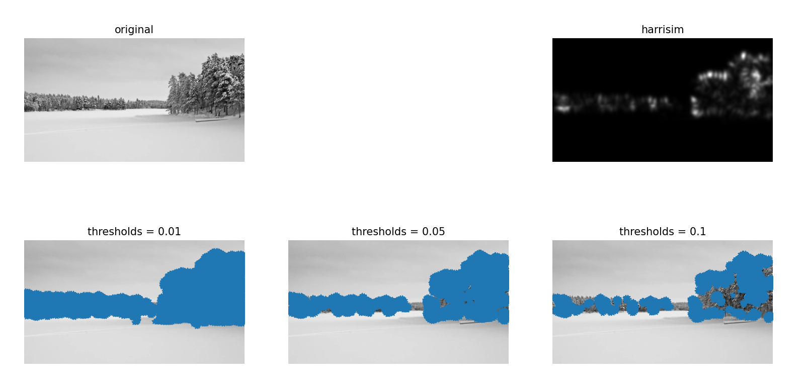
实验结果给出的图片来看,我们可以看到Harris响应函数的图片,min_dist即分割角点和图片边界的最少像素数目统一设为6,当阈值越低时符合条件的角点越多。不过min_dist小时,其显示也不怎么明显这里将min_dist设为30,效果图就为:
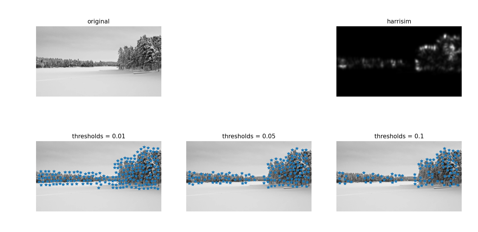
这样看来当min_dist越大时,角点代表的周围的邻近像素点越多,图像中显示的角点也就越发分散,更加清晰直观。
Harris算法的优点:
1、旋转不变性,椭圆转过一定角度但是其形状保持不变(特征值保持不变)
2、对于图像灰度的仿射变化具有部分的不变性,由于仅仅使用了图像的一介导数,对于图像灰度平移变化不变;对于图像灰度尺度变化不变
缺点:
1、对尺度很敏感,不具备几何尺度不变性。
2、提取的角点是像素级的
图像间寻找对应点
Harris角点检测器仅仅能够检测出图像中的兴趣点,但没有给出通过比较图像间的兴趣点来寻找匹配角点的方法。需要在每个点上加入描述子信息,并给出一个比较这些描述子的方法。
兴趣点描述子是分配给兴趣点的一个向量,描述该点附近的图像的表观信息,描述子越好,寻找到的对应点越好,用对应点或者对应来描述相同物体和场景点在不同图像上形成的像素点。
通常,两个相同大小的像素块的相关矩阵定义为:
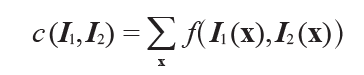
其中,函数f随着相关方法的变化而变化。上式取像素块中所有像素位置x的和。对于互相关矩阵,函数,因此,
,
值越大,两个像素块的相似度越高。
归一化的互相关矩阵:
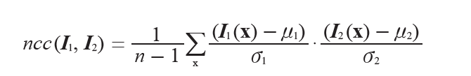
n为像素块中像素的数目,表示为每个像素块中的平均像素值强度,
表示为每个像素块中的标准差。通过减去均值和除以标准差,该方法对图像亮度变化具有稳健性。
实验代码如下:
# 图像间寻找对应点
from PIL import Image
from numpy import *
from pylab import *
from scipy.ndimage import filters
from imtools import harris_points, harris_response


# 为获得图像像素块,并使用归一化的互相关矩阵来比较需要以下函数
def get_descriptor(image, filtered_coords, wid=5):
    """
    对于每个返回的点,返回点周围2*wid+1个像素的值(假设选取点的min_distance > wid0)
    :param image: 原图
    :param filtered_coords:角点
    :param wid:
    :return:
    """
    desc = []
    for coords in filtered_coords:
        patch = image[coords[0] - wid:coords[0]+wid+1,
        coords[1] - wid:coords[1]+wid+1].flatten()
        desc.append(patch)
    return desc


def match(desc1, desc2, threshold=0.5):
    """
    对于第一幅图像中的每个角点描述子,使用归一化回香港,选取它在第二幅图像中的匹配角点
    :param desc1:
    :param desc2:
    :param threshold:
    :return:
    """
    n = len(desc1[0])
    # 点对的距离
    d = -ones((len(desc1), len(desc2)))
    for i in range(len(desc1)):
        for j in range(len(desc2)):
            d1 = (desc1[i] - mean(desc1[i])) / std(desc1[i])
            d2 = (desc2[j] - mean(desc2[j])) / std(desc2[j])
            ncc_value = sum(d1 * d2) / (n-1)
            if ncc_value > threshold:
                d[i, j] = ncc_value
    # 排序
    ndx = argsort(-d)
    matchscores = ndx[:, 0]
    return matchscores


def match_twosided(desc1, desc2, threshold=0.5):
    """
    两边对称版本的match()
    :param desc1:
    :param desc2:
    :param threshold: 阈值
    :return:
    """
    matches_12 = match(desc1, desc2, threshold)
    matches_21 = match(desc2, desc1, threshold)
    ndx_12 = where(matches_12 >= 0)[0]
    # 去除非对称的匹配
    for n in ndx_12:
        if matches_21[matches_12[n]] != n:
            matches_12[n] = -1
    return matches_12


def appendimages(img1, img2):
    """
    :param img1: 图片1
    :param img2: 图片2
    :return: 返回将两幅图像并排接为一幅新图像
    """
    row1 = img1.shape[0]
    row2 = img2.shape[0]
    if row1 < row2:
        img1 = concatenate((img1, zeros((row2 - row1, img1.shape[1]))), axis=0)
    elif row2 < row1:
        img2 = concatenate((img2, zeros((row1 - row2, img2.shape[1]))), axis=0)
    return concatenate((img1, img2), axis=1)


def plot_matches(img1, img2, losc1, losc2, matchscores, show_below=True):
    """
    显示一幅带有连接匹配之间连线的图片
    :param img1: 数组图像1
    :param img2: 数组图像2
    :param losc1: 特征位置
    :param losc2: 特征位置
    :param matchscores: match()的输出
    :param show_below:
    :return:
    """
    img3 = appendimages(img1, img2)
    if show_below:
        # vstack()将两个数组堆叠成一列
        img3 = vstack((img3, img3))
    imshow(img3)
    cols1 = img1.shape[1]
    for i, m in enumerate(matchscores):
        if m > 0:
            plot([losc1[i][1], losc2[m][1] + cols1],
                 [losc1[i][0], losc2[m][0]], 'c')
    axis('off')

wid = 5
img1 = array(Image.open('D:\\picture\\11.jpg').convert('L'))
img2 = array(Image.open('D:\\picture\\12.jpg').convert('L'))
# 响应函数,高斯滤波器的sigma为5
harrisimg = harris_response(img1, 5)
filtered_coords1 = harris_points(harrisimg, wid+1)
d1 = get_descriptor(img1, filtered_coords1, wid)

harrisimg = harris_response(img2, 5)
filtered_coords2 = harris_points(harrisimg, wid+1)
d2 = get_descriptor(img2, filtered_coords2, wid)
print('start matching')
matches = match_twosided(d1, d2)
figure()
gray()
plot_matches(img1, img2, filtered_coords1, filtered_coords2, matches)
show()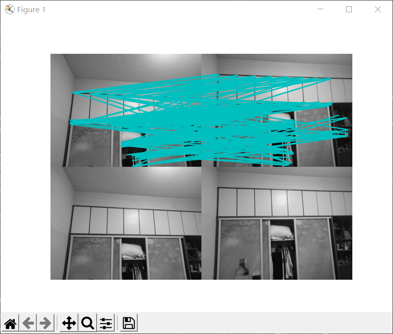
实验结果得出了两幅图像相匹配得到的对应角点,函数get_descriptor的参数为奇数大小长度的方形灰度图像块,该图像块的中心点位处理的像素点。函数的作用的将图像的像素值压平成一个向量,如何添加到描述子列表中。第二个函数match使用归一化的互相关矩阵,将每个描述子匹配到另一个图像中的最优候选点。函数match_twosided通过在两边分别绘制出图像,使用线段连接匹配的像素点来直观地可视化。
缺点:这个算法存在着一些不正确的匹配,这是由于图像像素块的互相关矩阵具有较弱的描述性。
二、SIFT(尺度不变特征变换)
SIFT特征包含兴趣点检测器和描述子,且其描述子具有非常强的稳健性,如今SIFT描述符经常和许多不同的兴趣点检测器相结合使用,有时甚至在整幅图像上密集地使用,SIFT特征对于尺度、旋转和亮度都具有不变性,因此可用于三维视角和噪声的可靠匹配。
2.1 兴趣点
SIFT特征使用高斯差分函数来定位兴趣点:
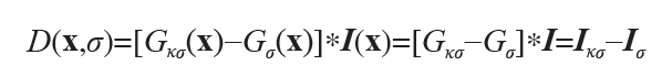
其中,是使用
模糊的灰度图像,k是决定相差尺度的常数。兴趣点是在图像位置和尺度变化下
的最大值和最小值点。这些候选位置点通过滤波去除不稳定点。
2.2 描述子
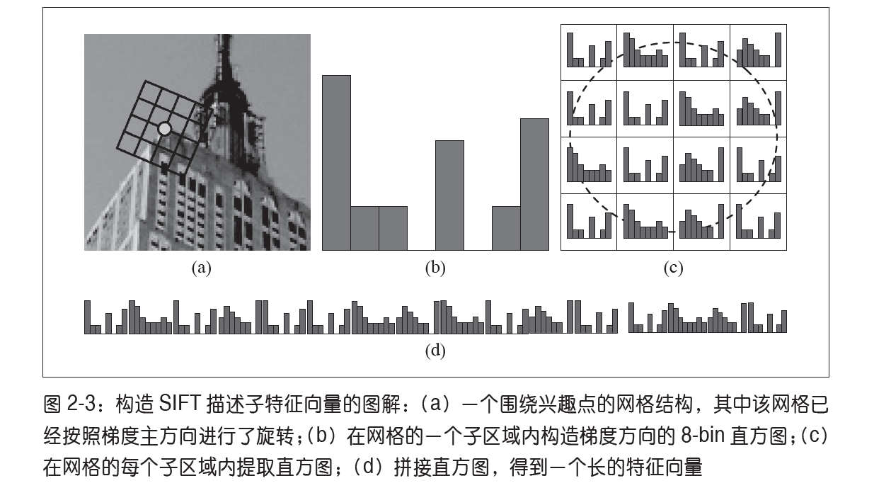
描述子给出了兴趣点的位置和尺度信息。为了实现旋转不变性,基于每个点周围图像梯度的方向和大小,SIFT描述子又引入了参考方向。SIFT描述子使用主方向描述参考方向,主方向使用方向直方图来度量。
为了使图像亮度具有稳健性,要使用图像梯度,描述子在每个像素点附近选取子区域网络并在每个子区域内计算图像梯度方向直方图。每个子区域的直方图拼接后就组成了描述子向量。一般将描述子的标准设置位使用4*4的子区域,每个子区域使用8给小区间的方向直方图,由此就会产生128个小区间的直方图。
2.3 检测兴趣点
由于用python实现SIFT特征的所有步骤的效率不高,因此使用开源工具包VLFeat提供的二进制文件来计算图像的SIFT特征,工具包可以在http://www.vlfeat.org/下载。这里开始我使用了开源工具包,因此在代码上可能与上面的内容有所出入。
因为二进制文件需要的图像格式为灰度.pgm,所以在执行前需要将图片的格式进行转化代码如下:
def process_image(imagename,resultname,params="--edge-thresh 10 --peak-thresh 5"):
    """ 处理图像并将结果保存在文件里 """

    if imagename[-3:] != 'pgm':
        # create a pgm file
        im = Image.open(imagename).convert('L')
        im.save('tmp.pgm')
        imagename = 'tmp.pgm'

    cmmd = str("D:\load\\vlfeat-0.9.20-bin\\vlfeat-0.9.20\\bin\win64\sift.exe "+imagename+" --output="+resultname+
                " "+params)
    os.system(cmmd)
    print ('processed', imagename, 'to', resultname)
cmmd中的代码为解压后的vlfeat文件里sift.exe所在地址。接下来就是从上面的输出文件里将特征读取到Numpy数组中的函数,具体代码如下:
def read_features_from_file(filename):
    """ 读取特征属性值,然后将其以矩阵的形式返回 """

    f = loadtxt(filename)
    return f[:,:4],f[:,4:] # feature locations, descriptors
在读取特征后,就需要通过于图像中绘制出它们的位置,以实现可视化。
def plot_features(im,locs,circle=False):
    """ 显示带有特征的图像 """

    def draw_circle(c,r):
        t = arange(0,1.01,.01)*2*pi
        x = r*cos(t) + c[0]
        y = r*sin(t) + c[1]
        plot(x,y,'b',linewidth=2)

    imshow(im)
    if circle:
        for p in locs:
            draw_circle(p[:2],p[2])
    else:
        plot(locs[:,0],locs[:,1],'ob')
    axis('off')
最后的主程序运行:
from PCV.localdescriptors import sift, harris
from PIL import Image
from pylab import *
imgname = 'D:\\picture\\11.jpg'
img1 = array(Image.open(imgname).convert('L'))
gray()
# SIFT特征
sift.process_image(imgname, 'empire.sift')
l1, d1 = sift.read_features_from_file('empire.sift')
# 角点检测
harrisimg = harris.compute_harris_response(img1)
filtered_coords = harris.get_harris_points(harrisimg, 6)
# 图片输出
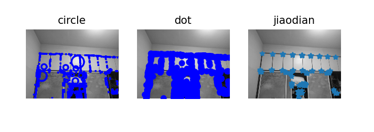
subplot(131)
sift.plot_features(img1, l1, circle=True), title('circle')
subplot(132)
sift.plot_features(img1, l1, circle=False), title('dot')
subplot(133)
harris.plot_harris_points(img1, filtered_coords)
show()输出图像见下图,可以看出harris角点和SIFT特征两种算法选择特征点位置不同。
2.4 匹配描述子
对于将一幅图像中的特征匹配到另一幅图像的特征,一种由Lowe提出的稳健准则是使用这两个特征距离和两个最匹配特征距离的比率,该准则保证能够找到足够相似的唯一特征,可以大大降低错误的匹配数。
下面给出匹配描述子和图像对应点两种方法的对比:
from PIL import Image
from pylab import *
import sys
from PCV.localdescriptors import sift

if len(sys.argv) >= 3:
    im1f, im2f = sys.argv[1], sys.argv[2]
else:
    im1f = 'D:\\picture\\test_img0\\tem1.jpg'
    im2f = 'D:\\picture\\test_img0\\tem2.jpg'
im1 = array(Image.open(im1f))
im2 = array(Image.open(im2f))
sift.process_image(im1f, 'out_sift_1.txt')
l1, d1 = sift.read_features_from_file('out_sift_1.txt')
figure()
gray()
subplot(121)
sift.plot_features(im1, l1, circle=False)
sift.process_image(im2f, 'out_sift_2.txt')
l2, d2 = sift.read_features_from_file('out_sift_2.txt')
subplot(122)
sift.plot_features(im2, l2, circle=False)
matches = sift.match_twosided(d1, d2)
print('{} matches'.format(len(matches.nonzero()[0])))
figure()
gray()
sift.plot_matches(im1, im2, l1, l2, matches, show_below=True)
show()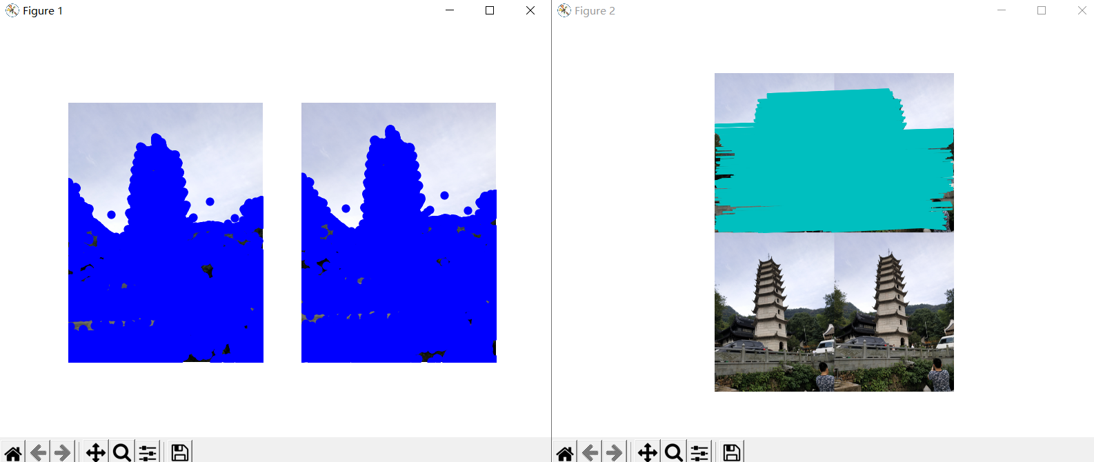
观察SIFT特征和对应点两种方法分别得出的图,可以看出相比于对应点而言SIFT描述子的错误更少一点,SIFT算法的其实就是在不同尺度上查找特征点并计算出其方向。
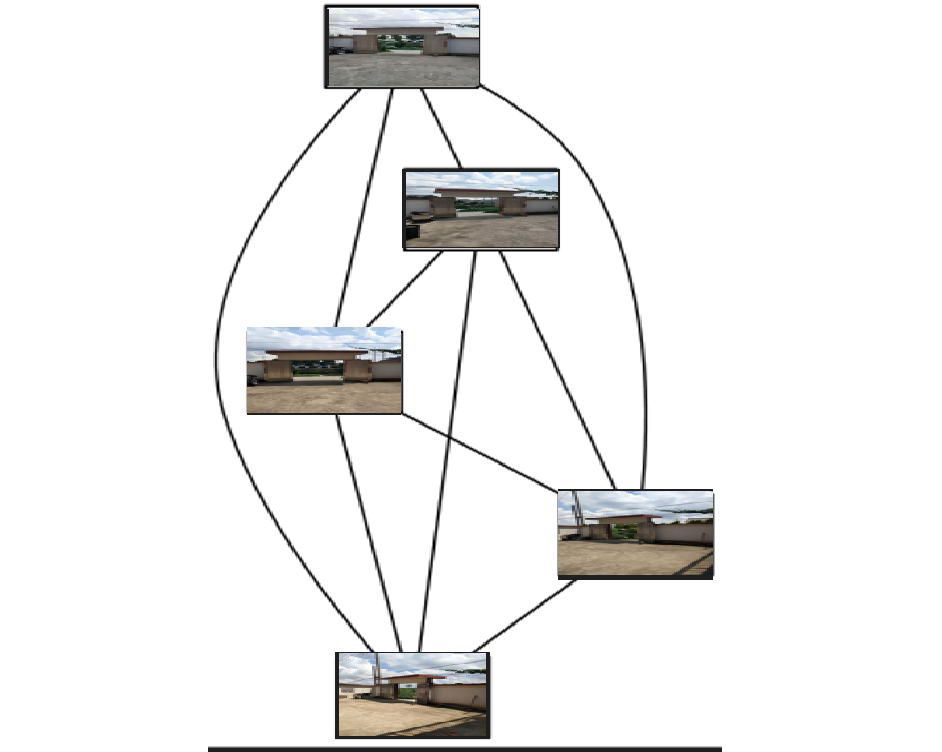
2.3 匹配地理标记图像可视化连接的图像
首先需要通过图像间是否具有匹配的局部描述子来定义图像间的连接,然后可视化这些连接情况,这里要使用到pydot工具包。
pydot使用GraphViz和Pyprasing,这里需要提前进行安装,否则将会显示无法找到neato。
具体的安装可以参考
Windows10(64位)下快速安装 pygraphviz_高精度计算机视觉的博客-CSDN博客
我是在anaconda3下进行安装GraphViz的,直接在pycharm的setting中安装的pydot并不能满足所有情况。
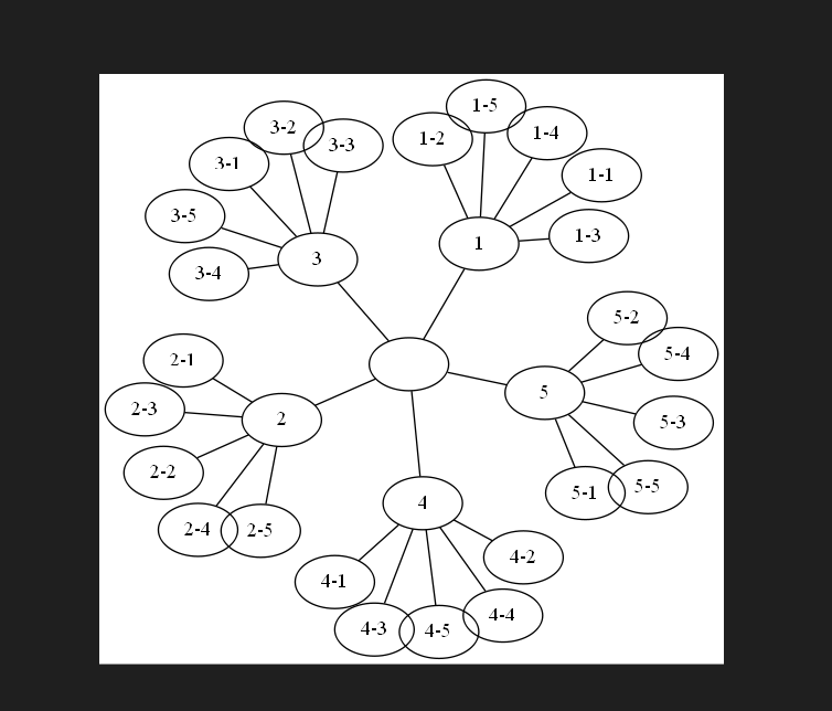
使用pydot工具包创建图示例:
import pydot
g = pydot.Dot(graph_type='graph')
g.add_node(pydot.Node(str(0),fontcolor='transparent'))
for i in range(5):
     g.add_node(pydot.Node(str(i+1)))
     g.add_edge(pydot.Edge(str(0),str(i+1)))
     for j in range(5):
         g.add_node(pydot.Node(str(j+1)+'-'+str(i+1)))
         g.add_edge(pydot.Edge(str(j+1)+'-'+str(i+1), str(j+1)))
g.write('graph.jpg', prog='neato')
结果:运行完后可以在项目文件内找到graph.jpg,打开即可。
错误:按照书中给出的代码最后得出的jpg图像显示格式存在问题无法显示,此时需要对g.write()进行更正。

将
g.write('graph.jpg', prog='neato')添上限制:
g.write('graph.jpg', prog='neato', format='png', encoding=None)此时就可以得到正确的图片了
接下来进行实验:
from PIL import Image
from PCV.localdescriptors import sift
import pydot
from pylab import *

path = "D:\\picture\\test_img3"
imlist = ('D:\\picture\\test_img3\\img1.jpg', 'D:\\picture\\test_img3\\img2.jpg',
          'D:\\picture\\test_img3\\img3.jpg', 'D:\\picture\\test_img3\\img4.jpg', 'D:\\picture\\test_img3\\img5.jpg')
nbr_images = len(imlist)
featlist = [imname[:-3] + 'sift' for imname in imlist]
for i, imname in enumerate(imlist):
    sift.process_image(imname, featlist[i])

matchscores = zeros((nbr_images, nbr_images))

for i in range(nbr_images):
    for j in range(i, nbr_images):
        print('comparing ', imlist[i], imlist[j])
        l1, d1 = sift.read_features_from_file(featlist[i])
        l2, d2 = sift.read_features_from_file(featlist[j])
        matches = sift.match_twosided(d1, d2)
        nbr_matches = sum(matches > 0)
        print('number of matches = ', nbr_matches)
        matchscores[i, j] = nbr_matches
print("The match scores is: \n", matchscores)

for i in range(nbr_images):
    for j in range(i + 1, nbr_images):  # no need to copy diagonal
        matchscores[j, i] = matchscores[i, j]

# 可视化
threshold = 2  # min number of matches needed to create link
g = pydot.Dot(graph_type='graph')  # don't want the default directed graph
for i in range(nbr_images):
    for j in range(i + 1, nbr_images):
        if matchscores[i, j] > threshold:
            # first image in pair
            im = Image.open(imlist[i])
            im.thumbnail((100, 100))
            filename = str(i) + '.png'
            im.save(filename)  # need temporary files of the right size
            g.add_node(pydot.Node(str(i), fontcolor='transparent', shape='rectangle', image=path + filename))
            # second image in pair
            im = Image.open(imlist[j])
            im.thumbnail((100, 100))
            filename = str(j) + '.png'
            im.save(filename)  # need temporary files of the right size
            g.add_node(pydot.Node(str(j), fontcolor='transparent', shape='rectangle', image=path + filename))
            g.add_edge(pydot.Edge(str(i), str(j)))
g.write_png('test1.png')
程序运行后:
processed tmp.pgm to D:\picture\test_img3\img1.sift
processed tmp.pgm to D:\picture\test_img3\img2.sift
processed tmp.pgm to D:\picture\test_img3\img3.sift
processed tmp.pgm to D:\picture\test_img3\img4.sift
processed tmp.pgm to D:\picture\test_img3\img5.sift
comparing  D:\picture\test_img3\img1.jpg D:\picture\test_img3\img1.jpg
number of matches =  16835
comparing  D:\picture\test_img3\img1.jpg D:\picture\test_img3\img2.jpg
number of matches =  17
comparing  D:\picture\test_img3\img1.jpg D:\picture\test_img3\img3.jpg
number of matches =  108
comparing  D:\picture\test_img3\img1.jpg D:\picture\test_img3\img4.jpg
number of matches =  27
comparing  D:\picture\test_img3\img1.jpg D:\picture\test_img3\img5.jpg
number of matches =  8
comparing  D:\picture\test_img3\img2.jpg D:\picture\test_img3\img2.jpg
number of matches =  20061
comparing  D:\picture\test_img3\img2.jpg D:\picture\test_img3\img3.jpg
number of matches =  77
comparing  D:\picture\test_img3\img2.jpg D:\picture\test_img3\img4.jpg
number of matches =  6
comparing  D:\picture\test_img3\img2.jpg D:\picture\test_img3\img5.jpg
number of matches =  6
comparing  D:\picture\test_img3\img3.jpg D:\picture\test_img3\img3.jpg
number of matches =  17455
comparing  D:\picture\test_img3\img3.jpg D:\picture\test_img3\img4.jpg
number of matches =  11
comparing  D:\picture\test_img3\img3.jpg D:\picture\test_img3\img5.jpg
number of matches =  7
comparing  D:\picture\test_img3\img4.jpg D:\picture\test_img3\img4.jpg
number of matches =  24712
comparing  D:\picture\test_img3\img4.jpg D:\picture\test_img3\img5.jpg
number of matches =  241
comparing  D:\picture\test_img3\img5.jpg D:\picture\test_img3\img5.jpg
number of matches =  20092
The match scores is:
 [[1.6835e+04 1.7000e+01 1.0800e+02 2.7000e+01 8.0000e+00]
 [0.0000e+00 2.0061e+04 7.7000e+01 6.0000e+00 6.0000e+00]
 [0.0000e+00 0.0000e+00 1.7455e+04 1.1000e+01 7.0000e+00]
 [0.0000e+00 0.0000e+00 0.0000e+00 2.4712e+04 2.4100e+02]
 [0.0000e+00 0.0000e+00 0.0000e+00 0.0000e+00 2.0092e+04]]

Process finished with exit code 0
三、总结
本章的学习过程中遇到了很多困难,程序代码的理解还是不太清晰,在进行SIFT特征的学习时,因为工具包的安装问题导致消耗了很长时间。相关内容还需进一步加强理解。


 4414
4414


 被折叠的 条评论
为什么被折叠?
被折叠的 条评论
为什么被折叠?
 到【灌水乐园】发言


