Centernet 个人理解笔记

一，Centernet骨干网络之DLASeg

1，DLA34-base结构

代码块：

self.level0 = self._make_conv_level(
            channels[0], channels[0], levels[0])
self.level1 = self._make_conv_level(
            channels[0], channels[1], levels[1], stride=2)
self.level2 = Tree(levels[2], block, channels[1], channels[2], 2,
                           level_root=False,
                           root_residual=residual_root)
self.level3 = Tree(levels[3], block, channels[2], channels[3], 2,
                           level_root=True, root_residual=residual_root)
self.level4 = Tree(levels[4], block, channels[3], channels[4], 2,
                           level_root=True, root_residual=residual_root)
self.level5 = Tree(levels[5], block, channels[4], channels[5], 2,
                           level_root=True, root_residual=residual_root)

其中，level0 是上图第一个黑色框，level1是上图中第二个黑色框，level2到level5分别是上图从左到右4个红框，表示level=[1,2,2,1]的4棵树。
1）黑色框（conv Block）
代码块：

def _make_conv_level(self, inplanes, planes, convs, stride=1, dilation=1):
        modules = []
        for i in range(convs):
            modules.extend([
                nn.Conv2d(inplanes, planes, kernel_size=3,
                          stride=stride if i == 0 else 1,
                          padding=dilation, bias=False, dilation=dilation),
                BatchNorm(planes),
                nn.ReLU(inplace=True)])
            inplanes = planes
        return nn.Sequential(*modules)

结构：

2）绿色框（ Aggregation Node）
绿色框是连接2棵树的根节点， forward 函数中接受的是多个对象，用来聚合多个层的信
息，实现：

class Root(nn.Module):
    def __init__(self, in_channels, out_channels, kernel_size, residual):
        super(Root, self).__init__()
        self.conv = nn.Conv2d(
            in_channels, out_channels, 1,
            stride=1, bias=False, padding=(kernel_size - 1) // 2)
        self.bn = BatchNorm(out_channels)
        self.relu = nn.ReLU(inplace=True)
        self.residual = residual

    def forward(self, *x):
        children = x
        x = self.conv(torch.cat(x, 1))
        x = self.bn(x)
        if self.residual:
            x += children[0]
        x = self.relu(x)

        return x

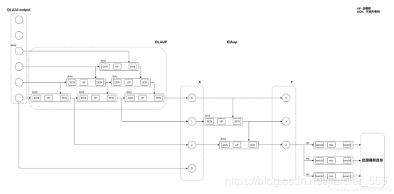
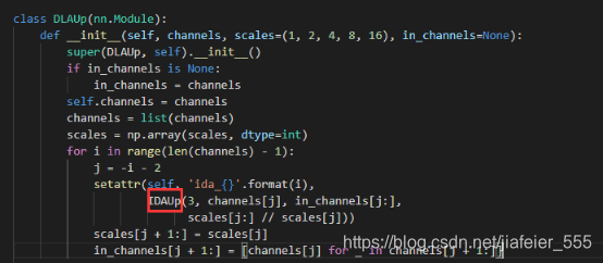
2，DLAUP结构
DLAup本身就是多个IDAup的组合。


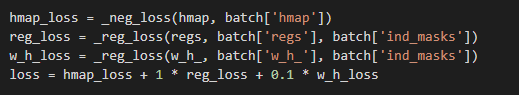
二，Centernet loss

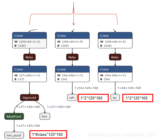
centernet模型输出由3部分组成，分别为hm_head,wh_head,reg_head，故而centernt loss也是由3部分组成，分别为预测类别热力图loss ，预测长宽的loss，以及预测偏移的loss。
并且3种损失权重不一样。

① hm_loss：
1）公式及其原理：

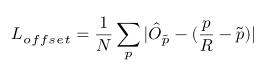
经验值：α = 2 and β = 4
Yxyc表示ground true 的热力图，即heatmap_gt，Yxyc=1，表示标注框的中心点位置。



实现：

def _neg_loss(pred, gt):
    ''' Modified focal loss. Exactly the same as CornerNet.
        Runs faster and costs a little bit more memory
      Arguments:
        pred (batch x c x h x w)
        gt_regr (batch x c x h x w)
    '''
    pos_inds = gt.eq(1).float()    #gt等于1的像素索引，前景
    neg_inds = gt.lt(1).float()    #gt小于1的像素索引，背景

    neg_weights = torch.pow(1 - gt, 4)   #背景loss惩罚式

    loss = 0

    pos_loss = torch.log(pred) * torch.pow(1 - pred, 2) * pos_inds     #前景loss计算
    neg_loss = torch.log(1 - pred) * torch.pow(pred, 2) * neg_weights * neg_inds   #背景loss计算

    num_pos = pos_inds.float().sum()
    pos_loss = pos_loss.sum()
    neg_loss = neg_loss.sum()

    if num_pos == 0:
        loss = loss - neg_loss
    else:
        loss = loss - (pos_loss + neg_loss) / num_pos
    return loss

② reg_loss:
公式及原理：


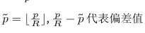
模型输出的featmap_pre是原图尺寸的1/R倍，一般R取4，所以将一个在原图尺寸的标注信息归一化到featmap_pre之后会存在一些小范围的偏移。
比如：一个在原图（10,10）像素点，下采样4倍之后，是2.5，然后向下取整，在featmap_pre上的左边是（2,2），如果我们再将其还原到原图中，则将会被还原到（8,8）上，这样在x,y方向均偏移了2个像素点。所以需要纠正。
③wh_loss:
公式及原理：

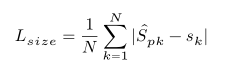
如果类k的标注框是（x1,y1,x2,y2）,那么Sk=（abs(x2-x1),abs(y2-y1)）
然后对网络输出进行L1Loss。

三，heatmap制作
1，高斯半径确定：
如果是训练点，线，即type是point,那么默认高斯半径是3，
如果是训练框，既type是cube,那么高斯半径由目标的高宽决定

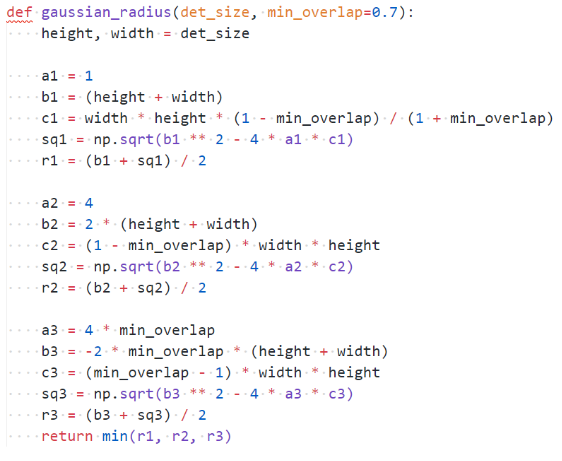
高斯核半径确定的问题由来：

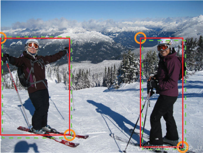
我们想让上图中红色标注框和绿色预测框最大程度的重叠，使两者IOU大于0.7。
那么此时，这两个框的位置最多会有以下三种情况：

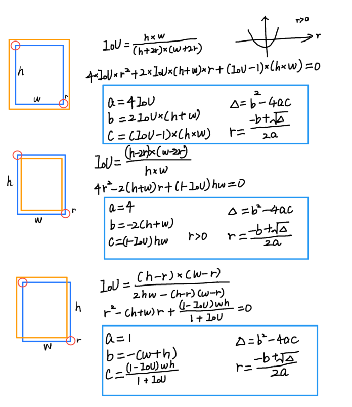
2，通过高斯半径产生二维高斯核，
3，根据当前框对应的类别，把高斯核覆盖到对应框中心在Heatmap上对应的位置。