NumPy库---Python数据分析和展示1（北理工mooc）

NumPy库

NumPy库入门

列表和数组的区别：

• 列表中元素类型可以不同，但数组中的元素必须类型相同

NumPy库的数组对象

开源的Python科学计算基础库。
ndarray数组对象：

• 可以去掉元素间运算所需的循环，是一维向量更像单个数据。
• 设置专门的数组对象，经过优化，可以提升运算速度。
• 有利于节省运算和存储空间。
  ndarray由两部分构成：
• 实际数据
• 描述其的元数据（数据维度，数据类型等）
  ndarray的别名为array，因此可以使用array生成数组如：

>>> import numpy as np
>>> a = np.array([[1, 2, 3, 4],[4, 5, 6, 7]])
>>> print(a)
[[1 2 3 4]
[4 5 6 7]]
>>> a.ndim
2
>>> a.shape
(2, 4)
>>> a.size
8
>>> a.dtype
dtype('int32')
>>> a.itemsize
4

轴（axis）：保存数据的维度
秩（rank）：轴的数量
ndarray的属性：

ndarray元素类型：

ndarray数组创建方法

1. 从列表、元组（可以混合）等类型创建数组：

x = np.array(list/tuple)
x = np.array(list/tuple, dtype=np.float32)
>>> x = np.array([[1, 2], [3, 4], (1, 2)])
>>> print(x)
[[1 2]
 [3 4]
 [1 2]]

2. 使用NumPy中的函数创建数组：
   
   
   

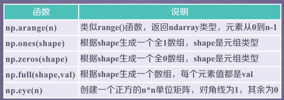
>>> np.arange(10) # 整数类型
array([0, 1, 2, 3, 4, 5, 6, 7, 8, 9])
>>> np.ones((3,6)) # 浮点数类型
array([[1., 1., 1., 1., 1., 1.],
       [1., 1., 1., 1., 1., 1.],
       [1., 1., 1., 1., 1., 1.]])
>>> np.zeros((3,6)) # 浮点数类型
array([[0., 0., 0., 0., 0., 0.],
       [0., 0., 0., 0., 0., 0.],
       [0., 0., 0., 0., 0., 0.]])
>>> np.eye(5) # 浮点数类型
array([[1., 0., 0., 0., 0.],
       [0., 1., 0., 0., 0.],
       [0., 0., 1., 0., 0.],
       [0., 0., 0., 1., 0.],
       [0., 0., 0., 0., 1.]])
>>> x = np.ones((2,3,4))
>>> print(x)
[[[1. 1. 1. 1.]
  [1. 1. 1. 1.]
  [1. 1. 1. 1.]]
  
 [[1. 1. 1. 1.]
  [1. 1. 1. 1.]
  [1. 1. 1. 1.]]]
>>> a = np.linspace(1, 10, 4) # np.linspace(起始值，结束值，元素个数)
>>> a
array([ 1.,  4.,  7., 10.])
>>> b = array([1, 2, 3,4])
Traceback (most recent call last):
  File "<stdin>", line 1, in <module>
NameError: name 'array' is not defined
>>> b = np.array([1,2,3,4])
>>> np.concatenate((a,b)) # 合并数组
array([ 1.,  4.,  7., 10.,  1.,  2.,  3.,  4.])

np.linspace有一个endpoint参数，不设置该参数时，最后一元素必为结束值，设置endpoint=false时，则最后一位部位结束值。
ndarray数组变换：

resize会生成新的数组，但reshape不会。

>>> a = np.ones((2, 3, 4),dtype=np.int32)
>>> a
array([[[1, 1, 1, 1],
        [1, 1, 1, 1],
        [1, 1, 1, 1]],
        
       [[1, 1, 1, 1],
        [1, 1, 1, 1],
        [1, 1, 1, 1]]])
>>> a.reshape((3,8))
array([[1, 1, 1, 1, 1, 1, 1, 1],
       [1, 1, 1, 1, 1, 1, 1, 1],
       [1, 1, 1, 1, 1, 1, 1, 1]])
>>> a.flatten()
array([1, 1, 1, 1, 1, 1, 1, 1, 1, 1, 1, 1, 1, 1, 1, 1, 1, 1, 1, 1, 1, 1,
       1, 1])
>>> a.astype(np.float) # 整数类型转换为了浮点数，且该方法会形成新的数组
array([[[1., 1., 1., 1.],
        [1., 1., 1., 1.],
        [1., 1., 1., 1.]],

       [[1., 1., 1., 1.],
        [1., 1., 1., 1.],
        [1., 1., 1., 1.]]])

>>> x = a.reshape((3,8))
>>> x
array([[1, 1, 1, 1, 1, 1, 1, 1],
       [1, 1, 1, 1, 1, 1, 1, 1],
       [1, 1, 1, 1, 1, 1, 1, 1]])
>>> a
array([[[1, 1, 1, 1],
        [1, 1, 1, 1],
        [1, 1, 1, 1]],

       [[1, 1, 1, 1],
        [1, 1, 1, 1],
        [1, 1, 1, 1]]])
>>> x = a.resize((3,8))
>>> x
>>> a
array([[1, 1, 1, 1, 1, 1, 1, 1],
       [1, 1, 1, 1, 1, 1, 1, 1],
       [1, 1, 1, 1, 1, 1, 1, 1]])
>>> a.tolist() # 数组转化为列表
[[1, 1, 1, 1, 1, 1, 1, 1], [1, 1, 1, 1, 1, 1, 1, 1], [1, 1, 1, 1, 1, 1, 1, 1]]
```python
**ndarray数组的操作：**
一维数组的索引和切片和列表类似。
 多维数组的索引与切片：
 ```python
>>> a
array([[[ 0,  1,  2,  3],
        [ 4,  5,  6,  7],
        [ 8,  9, 10, 11]],

       [[12, 13, 14, 15],
        [16, 17, 18, 19],
        [20, 21, 22, 23]]])
>>> a[1, 2, 3]
23
>>> a[0, 1, 2]
6
>>> a[-1, -2, -3]
17
>>> a[:, 1, -3]
array([ 5, 17])
>>> a[:, 1:3, :]
array([[[ 4,  5,  6,  7],
        [ 8,  9, 10, 11]],

       [[16, 17, 18, 19],
        [20, 21, 22, 23]]])
>>> a[:, :, ::2]
array([[[ 0,  2],
        [ 4,  6],
        [ 8, 10]],

       [[12, 14],
        [16, 18],
        [20, 22]]])

ndarray数组运算：

>>> a = np.arange(24).reshape((3, 8))
>>> a
array([[ 0,  1,  2,  3,  4,  5,  6,  7],
       [ 8,  9, 10, 11, 12, 13, 14, 15],
       [16, 17, 18, 19, 20, 21, 22, 23]])
>>> a.mean()
11.5
>>> a/a.mean()
array([[0.        , 0.08695652, 0.17391304, 0.26086957, 0.34782609,
        0.43478261, 0.52173913, 0.60869565],
       [0.69565217, 0.7826087 , 0.86956522, 0.95652174, 1.04347826,
        1.13043478, 1.2173913 , 1.30434783],
       [1.39130435, 1.47826087, 1.56521739, 1.65217391, 1.73913043,
        1.82608696, 1.91304348, 2.        ]])

对数组中数据执行元素级运算：

ceiling为不小于参数的最小整数值，floor为不大于参数的最大整数值。

>>> a = np.arange(24).reshape((3, 8))
>>> a
array([[ 0,  1,  2,  3,  4,  5,  6,  7],
       [ 8,  9, 10, 11, 12, 13, 14, 15],
       [16, 17, 18, 19, 20, 21, 22, 23]])
>>> np.square(a)
array([[  0,   1,   4,   9,  16,  25,  36,  49],
       [ 64,  81, 100, 121, 144, 169, 196, 225],
       [256, 289, 324, 361, 400, 441, 484, 529]], dtype=int32)
>>> np.sqrt(a)
array([[0.        , 1.        , 1.41421356, 1.73205081, 2.        ,
        2.23606798, 2.44948974, 2.64575131],
       [2.82842712, 3.        , 3.16227766, 3.31662479, 3.46410162,
        3.60555128, 3.74165739, 3.87298335],
       [4.        , 4.12310563, 4.24264069, 4.35889894, 4.47213595,
        4.58257569, 4.69041576, 4.79583152]])
>>> np.modf(a)
(array([[0., 0., 0., 0., 0., 0., 0., 0.],
       [0., 0., 0., 0., 0., 0., 0., 0.],
       [0., 0., 0., 0., 0., 0., 0., 0.]]), array([[ 0.,  1.,  2.,  3.,  4.,  5.,  6.,  7.],
       [ 8.,  9., 10., 11., 12., 13., 14., 15.],
       [16., 17., 18., 19., 20., 21., 22., 23.]]))
>>> np.modf(np.sqrt(a)) # 生成两个数组，区分开数组中元素的整数部分和小数部分
(array([[0.        , 0.        , 0.41421356, 0.73205081, 0.        ,
        0.23606798, 0.44948974, 0.64575131],
       [0.82842712, 0.        , 0.16227766, 0.31662479, 0.46410162,
        0.60555128, 0.74165739, 0.87298335],
       [0.        , 0.12310563, 0.24264069, 0.35889894, 0.47213595,
        0.58257569, 0.69041576, 0.79583152]]), array([[0., 1., 1., 1., 2., 2., 2., 2.],
       [2., 3., 3., 3., 3., 3., 3., 3.],
       [4., 4., 4., 4., 4., 4., 4., 4.]]))

NumPy二元函数：

>>> a = np.arange(24).reshape((3, 8))
>>> b = np.sqrt(a)
>>> a
array([[ 0,  1,  2,  3,  4,  5,  6,  7],
       [ 8,  9, 10, 11, 12, 13, 14, 15],
       [16, 17, 18, 19, 20, 21, 22, 23]])
>>> b
array([[0.        , 1.        , 1.41421356, 1.73205081, 2.        ,
        2.23606798, 2.44948974, 2.64575131],
       [2.82842712, 3.        , 3.16227766, 3.31662479, 3.46410162,
        3.60555128, 3.74165739, 3.87298335],
       [4.        , 4.12310563, 4.24264069, 4.35889894, 4.47213595,
        4.58257569, 4.69041576, 4.79583152]])
>>> np.maximum(a, b) # 元素类型不同时，生成的元素为浮点数
array([[ 0.,  1.,  2.,  3.,  4.,  5.,  6.,  7.],
       [ 8.,  9., 10., 11., 12., 13., 14., 15.],
       [16., 17., 18., 19., 20., 21., 22., 23.]])
>>> a > b
array([[False, False,  True,  True,  True,  True,  True,  True],
       [ True,  True,  True,  True,  True,  True,  True,  True],
       [ True,  True,  True,  True,  True,  True,  True,  True]])

NumPy数据存取

csv的存取

写入：np.savetxt(frame, array, fmt=’%18e’, delimier=None)

• frame：文件、字符串或产生器，可以是.gz或.bz2的压缩文件。
• array：存入文件的数组。
• fmt：写入文件时使用的格，如：%d %.2f %.18e。
• delimiter：分隔字符串，默认是任何空格，在csv中需要改为逗号。
  读入：np.loadtxt(frame, dtype=np.float, delimiter=None, unpack=False)
• frame：文件、字符串等，同上。
• dtpye：数据类型，即将读入的数据视作的类型，可选
• delimiter：同上
• unpack：如果为True，读入属性将分别写入不同变量。

>>> a = np.arange(100).reshape(5, 20)
>>> np.savetxt('F:/a.csv', a, fmt='%d', delimiter=',')
>>> b = np.loadtxt('F:/a.csv', delimiter=',')
>>> b
array([[ 0.,  1.,  2.,  3.,  4.,  5.,  6.,  7.,  8.,  9., 10., 11., 12.,
        13., 14., 15., 16., 17., 18., 19.],
       [20., 21., 22., 23., 24., 25., 26., 27., 28., 29., 30., 31., 32.,
        33., 34., 35., 36., 37., 38., 39.],
       [40., 41., 42., 43., 44., 45., 46., 47., 48., 49., 50., 51., 52.,
        53., 54., 55., 56., 57., 58., 59.],
       [60., 61., 62., 63., 64., 65., 66., 67., 68., 69., 70., 71., 72.,
        73., 74., 75., 76., 77., 78., 79.],
       [80., 81., 82., 83., 84., 85., 86., 87., 88., 89., 90., 91., 92.,
        93., 94., 95., 96., 97., 98., 99.]])
>>> b = np.loadtxt('F:/a.csv', delimiter=',',dtype=np.int)
>>> b
array([[ 0,  1,  2,  3,  4,  5,  6,  7,  8,  9, 10, 11, 12, 13, 14, 15,
        16, 17, 18, 19],
       [20, 21, 22, 23, 24, 25, 26, 27, 28, 29, 30, 31, 32, 33, 34, 35,
        36, 37, 38, 39],
       [40, 41, 42, 43, 44, 45, 46, 47, 48, 49, 50, 51, 52, 53, 54, 55,
        56, 57, 58, 59],
       [60, 61, 62, 63, 64, 65, 66, 67, 68, 69, 70, 71, 72, 73, 74, 75,
        76, 77, 78, 79],
       [80, 81, 82, 83, 84, 85, 86, 87, 88, 89, 90, 91, 92, 93, 94, 95,
        96, 97, 98, 99]])

csv只能有效存储一维和二维数据。

任意维度数据存取

存储：a.tofile(frame, sep=’’, format=’%s’)

• frame：文件，字符串。
• sep：数据分割字符串，若为空串，则写入的文件为二进制。
• format：写入数据的格式。
  读取：np.fromfile(frame, dtype=float, count=-1,sep=’’)
• frame：同上。
• dtpye：读取的数据类型。
• count：读入元素个数，默认为-1，表示整个文件。
• 数据分隔字符串，空串表示写入文件为二进制。

>>> a = np.arange(100).reshape(5,10,2)
>>> a.tofile('F:/b.dat', sep=',', format='%d')
>>> c = np.fromfile('F:/b.dat',dtype=np.int,sep=',')
>>> c
array([ 0,  1,  2,  3,  4,  5,  6,  7,  8,  9, 10, 11, 12, 13, 14, 15, 16,
       17, 18, 19, 20, 21, 22, 23, 24, 25, 26, 27, 28, 29, 30, 31, 32, 33,
       34, 35, 36, 37, 38, 39, 40, 41, 42, 43, 44, 45, 46, 47, 48, 49, 50,
       51, 52, 53, 54, 55, 56, 57, 58, 59, 60, 61, 62, 63, 64, 65, 66, 67,
       68, 69, 70, 71, 72, 73, 74, 75, 76, 77, 78, 79, 80, 81, 82, 83, 84,
       85, 86, 87, 88, 89, 90, 91, 92, 93, 94, 95, 96, 97, 98, 99])

多维数据写入的文件用逗号分割时，以文本方式打开看不出来维度的信息，只能看到数据的排列，以二进制文件写入时，其中的信息无法直接识别。
多维数据读入时，由于失去了维度信息，因此要用reshape来还原其维度。一般数组的其他信息如维度、数据类型等会使用另一个文件来进行存储。

便捷文件存取

存储：np.save(fname,array)或np.savez(fname,array)

• fname：文件名，以.npy为扩展名，压缩名为.npz
• array：数组变量
  读取：np.load(fname)

NumPy的random子库

NumPy的统计函数

不输入轴axis则是对所有元素进行计算。
axis=1，在数组第二维度做运算；axis=0，在数组第一维度做运算，即数组的最外一层。

>>> import numpy as np
>>> a = np.arange(15).reshape(3, 5)
>>> a
array([[ 0,  1,  2,  3,  4],
       [ 5,  6,  7,  8,  9],
       [10, 11, 12, 13, 14]])
>>> np.mean(a)
7.0
>>> np.mean(a,axis=1)
array([ 2.,  7., 12.])
>>> np.mean(a,axis=0)
array([5., 6., 7., 8., 9.])
>>> np.sum(a)
105
>>> np.average(a, axis=0, weights=[10, 5, 1])
array([2.1875, 3.1875, 4.1875, 5.1875, 6.1875])
>>> np.std(a)
4.320493798938574
>>> np.var(a)
18.666666666666668

>>> b = np.arange(15, 0, -1).reshape(3, 5)
>>> b
array([[15, 14, 13, 12, 11],
       [10,  9,  8,  7,  6],
       [ 5,  4,  3,  2,  1]])
>>> np.max(b)
15
>>> np.min(b)
1
>>> np.argmax(b)
0
>>> np.unravel_index(np.argmax(b), b.shape)
(0, 0)
>>> np.ptp(b)
14
>>> np.median(b)
8.0

NumPy的梯度函数

>>> a = np.random.randint(0, 20, (5))
>>> a
array([13,  2, 16, 18, 17])
>>> np.gradient(a)
array([-11. ,   1.5,   8. ,   0.5,  -1. ])

存在两侧值时，如16，则grad=(18-2)/2=8
只存在单边值时，如17，则grad=(17-18)/1=-1

>>> c = np.random.randint(0, 50, (3, 5))
>>> c
array([[ 2,  5, 42, 26, 38],
       [45,  7,  5, 18, 34],
       [12, 43, 24, 33, 22]])
>>> np.gradient(c)
[array([[ 43. ,   2. , -37. ,  -8. ,  -4. ],
       [  5. ,  19. ,  -9. ,   3.5,  -8. ],
       [-33. ,  36. ,  19. ,  15. , -12. ]]), array([[  3. ,  20. ,  10.5,  -2. ,  12. ],
       [-38. , -20. ,   5.5,  14.5,  16. ],
       [ 31. ,   6. ,  -5. ,  -1. , -11. ]])]

对于多维数组，输出梯度的第一个数组为最外层维度的梯度，第二个数组是第二层维度的梯度······