


文章目录
神经网络学习
从数据中学习
指由数据自动决定权重参数的值
机器学习(深度学习)与神经网络:

过拟合:
只对某个数据集过度拟合的状态称为过拟合(over fitting)。避免过拟合也是机器学习的一个重要课题。
损失函数
神经网络以某个指标为线索寻找最优权重参数。神经网络的学习中所用的指标称为损失函数(loss function)。这个损失函数可以使用任意函数,但一般用均方误差和交叉熵误差等。
均方误差(mean squared error)
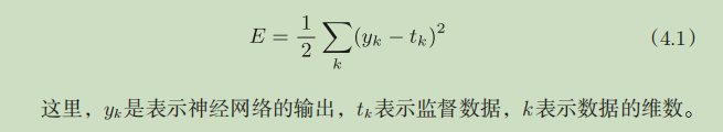
# 均方误差
def mean_squared_error(y, t):
    return 0.5 * np.sum((y - t) ** 2)
交叉熵误差(cross entropy error)

# 交叉熵误差
def cross_entropy_error(y0, t0):
    delta = 1e-7
    return -(np.sum(t0 * np.log(y0 + delta)))
加微小值是因为,np.log(0)会变成负无限大,后续无法计算。
mini-batch
# mini-batch
(x_train, t_train), (x_test, t_test) = load_mnist(one_hot_label=True)
train_size = x_train.shape[0]
batch_size = 20
mini_data_index = np.random.choice(train_size, batch_size)
mini_x_train = x_train[mini_data_index]
mini_t_train = t_train[mini_data_index]


# mini-batch的交叉熵误差
def mini_batch_cross_err(tnk, ynk):
    if ynk.ndim == 1:
        tnk = tnk.reshape(1, tnk.size)
        ynk = ynk.reshape(1, ynk.size)
    _batch = ynk.shape[0]
    return -np.sum(tnk * np.log(ynk + 1e-7)) / _batch


# 当监督数据是标签形式,即[2,7]这样的标签,非one-hot形式,可以表示为:
def mini_batch_cross_err_not_one_hot(tnk, ynk):
    if ynk.ndim == 1:
        tnk = tnk.reshape(1, tnk.size)
        ynk = ynk.reshape(1, ynk.size)
    _batch = ynk.shape[0]
    return -np.sum(np.log(y[np.arange(0, _batch), tnk] + 1e-7)) / _batch
y[np.arange(0, _batch), tnk]的说明:
y = np.array([[11,12,13,14,15],[21,22,23,24,25]])
y
array([[11, 12, 13, 14, 15],
       [21, 22, 23, 24, 25]])
y[0,1]
12
y[[0],[1]]
array([12])
y[[0,1],[1,1]]
array([12, 22])
数值微分
中心差分
def numerical_diff(f, x):
    h =1e-4
    return (f(x+h) - f(x-h)) / 2*h
偏导
我们把有多个变量的函数的导数称为偏导数。
问题1:f(x0,x1) = x0 ^ 2 + x1 ^ 2,求x0=3,x1=4时,关于x0的偏导数
>>> def function_tmp1(x0):
...     return x0*x0 + 4.0**2.0
...
>>> numerical_diff(function_tmp1, 3.0)
6.00000000000378
像这样,偏导数和单变量的导数一样,都是求某个地方的斜率。不过,
偏导数需要将多个变量中的某一个变量定为目标变量,并将其他变量固定为
某个值。在上例的代码中,为了将目标变量以外的变量固定到某些特定的值
上,我们定义了新函数。然后,对新定义的函数应用了之前的求数值微分的
函数,得到偏导数。
梯度
在刚才的例子中,我们按变量分别计算了x0和x1的偏导数。现在,我
们希望一起计算x0和x1的偏导数。比如,我们来考虑求x0=3,x1=4时(x0,x1)
的偏导数。由全部变量的偏导数汇总而成的向量称为梯度(gradient)。
梯度可以像下面这样来实现:
# 偏导 f(x1,x2)在[x,x`]的偏导
def numerical_gradient(f, x):
    grad = np.zeros_like(x)
    h = 1e-4

    for i in range(x.size):
        temp = x[i]
        x[i] = temp + h
        fh1 = f(x)

        x[i] = temp - h
        fh2 = f(x)

        grad[i] = (fh1 - fh2) / (2*h)
        x[i] = temp  # 还原x[i]

    return grad


# 测试
def fxy(x):
    return np.sum(x ** 2)


print(numerical_gradient(fxy, np.array([3.0, 4.0])))
print(numerical_gradient(fxy, np.array([0.0, 2.0])))
print(numerical_gradient(fxy, np.array([3.0, 0.0])))
'''结果:
[6. 8.]
[0. 4.]
[6. 0.]
'''
实际上,梯度会指向各点处的函数值降低的方向。更严格地讲,梯度指示的方向
是各点处的函数值减小最多的方向。这是一个非常重要的性质,请一定牢记!
梯度法
在梯度法中,函数的取值从当前位置沿着梯度方向前进一定距离,然后在新的地方重新求梯度,
再沿着新梯度方向前进,如此反复,不断地沿梯度方向前进。像这样,通过不断地沿梯度方向前进,
逐渐减小函数值的过程就是梯度法(gradient method)。
梯度法是解决机器学习中最优化问题的常用方法,特别是在神经网络的学习中经常被使用。

参数f是要进行最优化的函数,init_x是初始值,lr是学习率learning rate,step_num是梯度法的重复次数。
numerical_gradient(f,x)会求函数的梯度,用该梯度乘以学习率得到的值进行更新操作,由step_num指定重
复的次数。
import numpy as np
from numerical_gradient import numerical_gradient, fxy


# 梯度下降法
def gradient_descent(f, init_x, lr=0.01, step_num=100):
    x = init_x

    for i in range(step_num):
        grad = numerical_gradient(f, x)
        x -= lr * grad

    return x


# 测试
init_x_arg = np.array([-3.0, 4.0])
print(gradient_descent(fxy, init_x_arg, lr=0.1, step_num=100))

'''结果
[-6.11110793e-10  8.14814391e-10]
'''
神经网络的梯度
神经网络的学习也要求梯度。这里所说的梯度是指损失函数关于权重参数的梯度。

def gradient(f, x):
    h = 1e-4
    grad = np.zeros_like(x)
    it = np.nditer(x, flags=['multi_index'], op_flags=['readwrite'])
    while not it.finished:
        idx = it.multi_index
        temp = x[idx]
        x[idx] = temp + h
        f1 = f(x)
        x[idx] = temp - h
        f2 = f(x)
        grad[idx] = (f1 - f2) / (2 * h)
        x[idx] = temp
        it.iternext()
    return grad
import sys
import numpy as np
sys.path.append('../..')
from common.functions import softmax, cross_entropy_error
from gradient import gradient


# 神经网络的梯度
class SimpleNet:
    def __init__(self):
        self.W = np.random.randn(2, 3)  # 高斯分布初始化

    def predict(self, x):
        return np.dot(x, self.W)

    def loss(self, x, t):
        z = self.predict(x)
        y = softmax(z)
        return cross_entropy_error(y, t)


# 测试
net = SimpleNet()
print('W=', net.W)
x = np.array([0.6, 0.9])

p = net.predict(x)
print('p=', p)
print(np.argmax(p))

t = np.array([0, 0, 1])
loss = net.loss(x, t)
print('loss=', loss)


def f(w):
    return net.loss(x, t)


dW = gradient(f, net.W)
print(dW)

'''
W= [[-2.31451767 -0.35981419  0.48423579]
 [-0.40722287  0.60371311 -0.14211043]]
p= [-1.75521118  0.32745329  0.16264208]
1
loss= 0.8441895899451256
[[ 0.03789755  0.30415907 -0.34205661]
 [ 0.05684632  0.4562386  -0.51308492]]
'''
学习算法的实现
两层神经网络
# two_layer_net.py
import sys
sys.path.append('../..')
from common.functions import sigmoid, softmax, cross_entropy_error, numerical_gradient
import numpy as np


class TwoLayerNet:

    def __init__(self, input_size, hidden_size, output_size, weight_init_std=0.01):
        self.params = {
            'W1': weight_init_std * np.random.randn(input_size, hidden_size),
            'W2': weight_init_std * np.random.randn(hidden_size, output_size),
            'b1': np.zeros(hidden_size),
            'b2': np.zeros(output_size)
        }

    def predict(self, x):
        W1, W2 = self.params['W1'], self.params['W2']
        b1, b2 = self.params['b1'], self.params['b2']
        a1 = np.dot(x, W1) + b1
        z1 = sigmoid(a1)
        a2 = np.dot(z1, W2) + b2
        y = softmax(a2)
        return y

    def loss(self, x, t):
        y = self.predict(x)
        return cross_entropy_error(y, t)

    def accuracy(self, x, t):
        y = self.predict(x)
        y = np.argmax(y, axis=1)
        t = np.argmax(t, axis=1)
        accuracy = np.sum(y == t) / float(x.shape[0])
        return accuracy

    # x: 输入数据 t: 监督数据   梯度
    def numerical_gradient(self, x, t):
        def loss_func(W):
            return self.loss(x, t)

        W1, W2 = self.params['W1'], self.params['W2']
        b1, b2 = self.params['b1'], self.params['b2']
        grads = {
            'W1': numerical_gradient(loss_func, W1),
            'b1': numerical_gradient(loss_func, b1),
            'W2': numerical_gradient(loss_func, W2),
            'b2': numerical_gradient(loss_func, b2)
        }
        return grads


# 测试 隐藏层20神经元,输出层10个神经元
net = TwoLayerNet(input_size=784, hidden_size=20, output_size=10)
print('W1', net.params['W1'].shape)
print('W2', net.params['W2'].shape)
# 伪数据输入100笔
x = np.random.rand(100, 784)
y = net.predict(x)
# 伪正确解标签100笔
t = np.random.rand(100, 10)
# 梯度
grads = net.numerical_gradient(x, t)
print(grads['W1'].shape)
print(grads['b1'].shape)
print(grads['W2'].shape)
print(grads['b2'].shape)

'''
W1 (784, 20)
W2 (20, 10)
(784, 20)
(20,)
(20, 10)
(10,)
'''
mini-batch实现
以TowLayerNet类为对象,对使用MNIST数据集进行学习
# train_neuralnet.py
from two_layer_net import TwoLayerNet
import sys

sys.path.append('../..')
from dataset.mnist import load_mnist
import numpy as np
import matplotlib.pyplot as plt

# 数据集学习-参数更新
(x_train, t_train), (x_test, t_test) = load_mnist(one_hot_label=True)
net = TwoLayerNet(input_size=784, hidden_size=20, output_size=10)

train_loss_list = []
train_acc_list = []
test_acc_list = []

iter_num = 10000
train_size = x_train.shape[0]
batch_size = 100
learning_rate = 0.1

iter_per_epoch = max(train_size / batch_size, 1)

# 训练iter_num次
for i in range(iter_num):
    # 获取mini-batch 随机取batch_size条
    batch_idx = np.random.choice(train_size, batch_size)
    x_train_batch = x_train[batch_idx]
    t_train_batch = t_train[batch_idx]

    # 计算梯度
    grad = net.numerical_gradient(x_train_batch, t_train_batch)
    for key in ('W1', 'b1', 'W2', 'b2'):
        net.params[key] -= grad[key] * learning_rate

    loss = net.loss(x_train_batch, t_train_batch)
    train_loss_list.append(loss)

    if i % iter_per_epoch == 0:
        train_acc = net.accuracy(x_train, t_train)
        test_acc = net.accuracy(x_test, t_test)
        train_acc_list.append(train_acc)
        test_acc_list.append(test_acc)
        print('i, train_acc, test_acc | ', i, str(train_acc), str(test_acc))
过拟合:虽然训练数据中的数字图像能被正确辨别,但是不在训练数据中的数字图像却无法被识别的现象


 1171
1171


 被折叠的 条评论
为什么被折叠?
被折叠的 条评论
为什么被折叠?
 到【灌水乐园】发言


