


目录
1. ReLU激活函数概述
1.1 什么是激活函数?
激活函数是神经网络中的核心组件,它决定了神经元是否应该被"激活",即是否将输入信号传递到下一层。激活函数为神经网络引入了非线性特性,使其能够学习复杂模式。
1.2 ReLU的诞生背景
在ReLU出现之前,神经网络主要使用Sigmoid和Tanh等激活函数。但这些函数存在梯度消失问题,限制了深层网络的训练效果。ReLU的提出彻底改变了这一局面。
2. ReLU原理详解
2.1 基本数学定义
ReLU(Rectified Linear Unit) 的数学表达式极其简单:
f(x) = max(0, x)
或者分段函数形式:
        { 0,  if x < 0
f(x) =  {
        { x,  if x ≥ 0
2.2 函数特性分析
2.2.1 输出范围
-
输入为负:输出恒为0
-
输入为非负:输出等于输入
-
输出范围:[0, +∞)
2.2.2 导数计算
ReLU的导数同样简单:
        { 0,  if x < 0
f'(x) = {
        { 1,  if x > 0
在x=0处,导数理论上不存在,但在实际实现中通常将其定义为0或1。
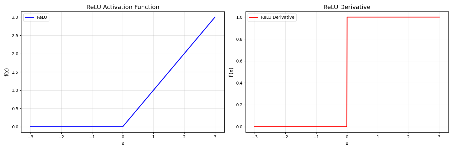
2.3 可视化理解
import numpy as np
import matplotlib.pyplot as plt

def relu(x):
    return np.maximum(0, x)

def relu_derivative(x):
    return np.where(x > 0, 1, 0)

# 生成数据
x = np.linspace(-3, 3, 1000)
y_relu = relu(x)
y_derivative = relu_derivative(x)

# 绘制图形
plt.figure(figsize=(15, 5))

plt.subplot(1, 2, 1)
plt.plot(x, y_relu, 'b-', linewidth=2, label='ReLU')
plt.title('ReLU激活函数', fontsize=14)
plt.xlabel('x', fontsize=12)
plt.ylabel('f(x)', fontsize=12)
plt.grid(True, alpha=0.3)
plt.legend()

plt.subplot(1, 2, 2)
plt.plot(x, y_derivative, 'r-', linewidth=2, label='ReLU导数')
plt.title('ReLU导数', fontsize=14)
plt.xlabel('x', fontsize=12)
plt.ylabel("f'(x)", fontsize=12)
plt.grid(True, alpha=0.3)
plt.legend()

plt.tight_layout()
plt.show()
运行代码得到下图
3. ReLU的优势与局限性
3.1 主要优势
3.1.1 缓解梯度消失问题
import numpy as np
import matplotlib.pyplot as plt

# ReLU函数定义
def relu(x):
    return np.maximum(0, x)

def relu_derivative_func(x):
    return np.where(x > 0, 1, 0)

# 对比不同激活函数的梯度
def compare_gradients():
    x = np.linspace(-5, 5, 1000)

    # Sigmoid及其导数
    sigmoid = 1 / (1 + np.exp(-x))
    sigmoid_derivative = sigmoid * (1 - sigmoid)

    # Tanh及其导数
    tanh_val = np.tanh(x)
    tanh_derivative = 1 - tanh_val**2

    # ReLU及其导数
    relu_val = relu(x)
    relu_derivative = relu_derivative_func(x)

    plt.figure(figsize=(12, 4))

    plt.subplot(1, 3, 1)
    plt.plot(x, sigmoid_derivative, 'r-', label='Sigmoid Derivative')
    plt.title('Sigmoid Derivative Range: (0, 0.25]')
    plt.grid(True, alpha=0.3)

    plt.subplot(1, 3, 2)
    plt.plot(x, tanh_derivative, 'g-', label='Tanh Derivative')
    plt.title('Tanh Derivative Range: (0, 1]')
    plt.grid(True, alpha=0.3)

    plt.subplot(1, 3, 3)
    plt.plot(x, relu_derivative, 'b-', label='ReLU Derivative')
    plt.title('ReLU Derivative Range: {0, 1}')
    plt.grid(True, alpha=0.3)
    plt.legend()

    plt.tight_layout()
    plt.show()

compare_gradients()
运行得到下图:
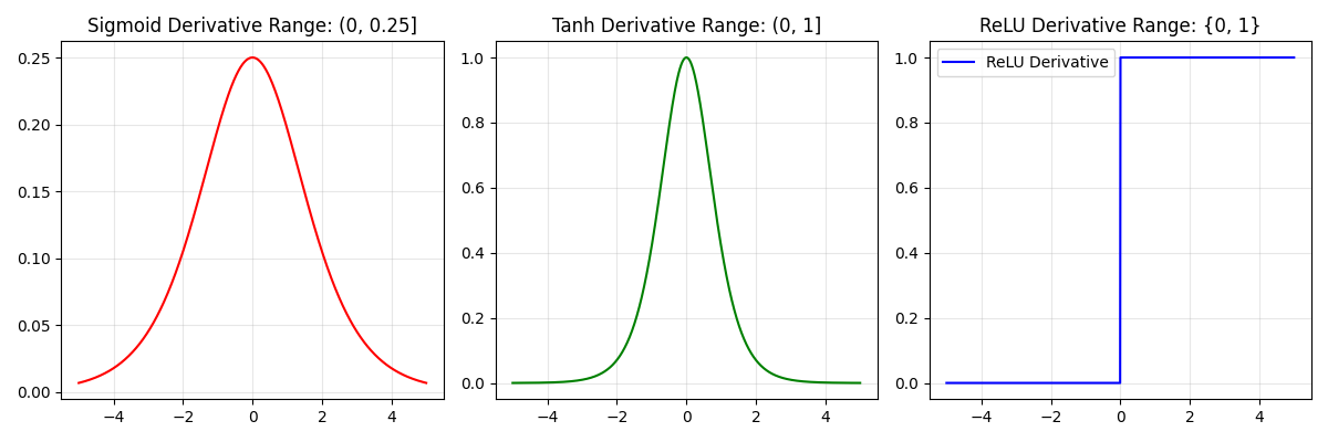
关键洞察:
-
Sigmoid导数最大为0.25,在深层网络中梯度会快速衰减
-
Tanh导数最大为1,但同样会衰减
-
ReLU在正区间的导数恒为1,彻底解决了梯度消失问题
3.1.2 计算效率极高
ReLU只涉及比较操作,没有指数、除法等复杂运算:
import time

def benchmark_activations():
    x = np.random.randn(1000000)

    # Sigmoid计算时间
    start = time.time()
    _ = 1 / (1 + np.exp(-x))
    sigmoid_time = time.time() - start

    # Tanh计算时间
    start = time.time()
    _ = np.tanh(x)
    tanh_time = time.time() - start

    # ReLU计算时间
    start = time.time()
    _ = np.maximum(0, x)
    relu_time = time.time() - start

    print(f"Sigmoid计算时间: {sigmoid_time:.6f}秒")
    print(f"Tanh计算时间: {tanh_time:.6f}秒")
    print(f"ReLU计算时间: {relu_time:.6f}秒")
    print(f"ReLU比Sigmoid快 {sigmoid_time/relu_time:.2f}倍")

benchmark_activations()
3.1.3 稀疏激活特性
ReLU的负半轴输出为0,使得网络具有稀疏性:
-
只有约50%的神经元被激活
-
减少参数间的相互依赖
-
增强模型的泛化能力
3.2 主要局限性
3.2.1 死亡ReLU问题(Dying ReLU)
def demonstrate_dying_relu():
    """演示死亡ReLU问题"""
    # 模拟权重更新导致神经元永久死亡的情况
    weights = np.array([-2.0, -1.5, -0.5, 0.5, 1.0, 2.0])
    inputs = np.array([1.0, 0.5, -0.2, 0.3, -0.8, 0.1])

    # 前向传播
    outputs = np.maximum(0, weights * inputs)

    print("权重:", weights)
    print("输入:", inputs)
    print("加权和:", weights * inputs)
    print("ReLU输出:", outputs)
    print("死亡神经元数量:", np.sum(outputs == 0))

demonstrate_dying_relu()
死亡ReLU的原因:
-
学习率过大
-
权重初始化不当
-
较大的负偏置
3.2.2 非零中心性
ReLU的输出始终≥0,这可能导致:
-
梯度更新方向单一
-
训练过程可能震荡
-
收敛速度受影响
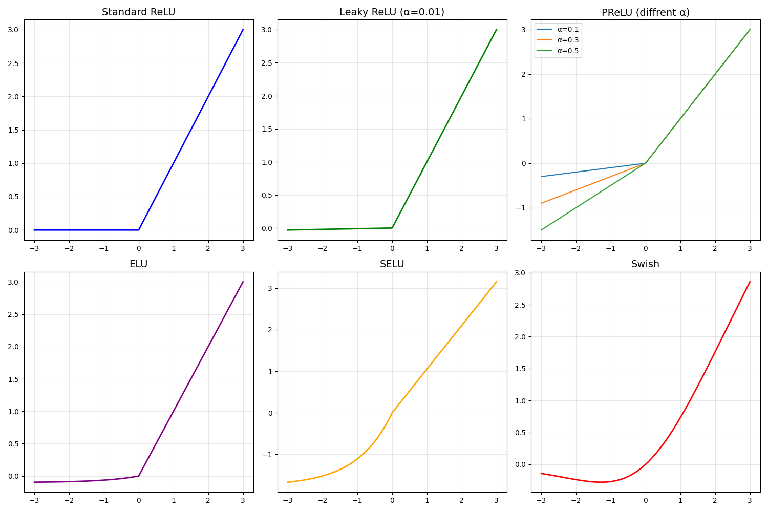
4. ReLU的变种改进
4.1 Leaky ReLU
import numpy as np
import matplotlib.pyplot as plt

def relu(x):
    return np.maximum(0, x)

def leaky_relu(x, alpha=0.01):
    return np.where(x > 0, x, alpha * x)

def plot_relu_variants():
    x = np.linspace(-3, 3, 1000)

    plt.figure(figsize=(15, 10))

    # ReLU
    plt.subplot(2, 3, 1)
    plt.plot(x, relu(x), 'b-', linewidth=2)
    plt.title('Standard ReLU', fontsize=14)
    plt.grid(True, alpha=0.3)

    # Leaky ReLU
    plt.subplot(2, 3, 2)
    plt.plot(x, leaky_relu(x), 'g-', linewidth=2)
    plt.title('Leaky ReLU (α=0.01)', fontsize=14)
    plt.grid(True, alpha=0.3)

    # PReLU (可学习参数的Leaky ReLU)
    plt.subplot(2, 3, 3)
    for alpha in [0.1, 0.3, 0.5]:
        plt.plot(x, leaky_relu(x, alpha), label=f'α={alpha}')
    plt.title('PReLU (diffrent α)', fontsize=14)
    plt.legend()
    plt.grid(True, alpha=0.3)

    # ELU
    plt.subplot(2, 3, 4)
    elu = np.where(x > 0, x, 0.1 * (np.exp(x) - 1))
    plt.plot(x, elu, 'purple', linewidth=2)
    plt.title('ELU', fontsize=14)
    plt.grid(True, alpha=0.3)

    # SELU
    plt.subplot(2, 3, 5)
    lam = 1.0507
    alpha = 1.67326
    selu = np.where(x > 0, lam * x, lam * alpha * (np.exp(x) - 1))
    plt.plot(x, selu, 'orange', linewidth=2)
    plt.title('SELU', fontsize=14)
    plt.grid(True, alpha=0.3)

    # Swish
    plt.subplot(2, 3, 6)
    swish = x * (1 / (1 + np.exp(-x)))
    plt.plot(x, swish, 'red', linewidth=2)
    plt.title('Swish', fontsize=14)
    plt.grid(True, alpha=0.3)

    plt.tight_layout()
    plt.show()

plot_relu_variants()
运行得到下图:
4.2 主要变种对比
| 变种名称 | 公式 | 优点 | 缺点 |
| Leaky ReLU | max(αx, x) | 解决死亡ReLU | 需要调参 |
| PReLU | max(αx, x) | α可学习 | 增加参数 |
| ELU | x if x>0 else α(eˣ-1) | 负区平滑 | 计算复杂 |
| SELU | λ×ELU | 自归一化 | 需要特定初始化 |
5. TensorFlow代码实现
5.1 基础ReLU实现
import tensorflow as tf
import numpy as np

class CustomReLU:
    """自定义ReLU实现"""

    @staticmethod
    def forward(x):
        """前向传播"""
        return tf.maximum(0.0, x)

    @staticmethod
    def backward(x, grad_output):
        """反向传播"""
        return tf.where(x > 0, grad_output, 0.0)

# 测试自定义ReLU
def test_custom_relu():
    # 创建测试数据
    x = tf.constant([-2.0, -1.0, 0.0, 1.0, 2.0])

    # 前向传播
    with tf.GradientTape() as tape:
        tape.watch(x)
        y = CustomReLU.forward(x)

    # 反向传播
    grad = tape.gradient(y, x)

    print("输入:", x.numpy())
    print("ReLU输出:", y.numpy())
    print("梯度:", grad.numpy())

test_custom_relu()
5.2 在神经网络中使用ReLU
def create_relu_network():
    """创建使用ReLU的神经网络"""

    # 方法1: 使用tf.nn.relu
    def create_with_tf_nn():
        model = tf.keras.Sequential([
            tf.keras.layers.Dense(128, input_shape=(784,)),
            tf.keras.layers.Lambda(lambda x: tf.nn.relu(x)),
            tf.keras.layers.Dense(64),
            tf.keras.layers.Lambda(lambda x: tf.nn.relu(x)),
            tf.keras.layers.Dense(10, activation='softmax')
        ])
        return model

    # 方法2: 直接在Dense层中指定activation
    def create_with_activation():
        model = tf.keras.Sequential([
            tf.keras.layers.Dense(128, activation='relu', input_shape=(784,)),
            tf.keras.layers.Dense(64, activation='relu'),
            tf.keras.layers.Dense(10, activation='softmax')
        ])
        return model

    # 方法3: 使用Leaky ReLU
    def create_with_leaky_relu():
        model = tf.keras.Sequential([
            tf.keras.layers.Dense(128, input_shape=(784,)),
            tf.keras.layers.LeakyReLU(alpha=0.01),
            tf.keras.layers.Dense(64),
            tf.keras.layers.LeakyReLU(alpha=0.01),
            tf.keras.layers.Dense(10, activation='softmax')
        ])
        return model

    # 方法4: 使用PReLU
    def create_with_prelu():
        model = tf.keras.Sequential([
            tf.keras.layers.Dense(128, input_shape=(784,)),
            tf.keras.layers.PReLU(),
            tf.keras.layers.Dense(64),
            tf.keras.layers.PReLU(),
            tf.keras.layers.Dense(10, activation='softmax')
        ])
        return model

    return {
        'tf_nn_relu': create_with_tf_nn(),
        'activation_relu': create_with_activation(),
        'leaky_relu': create_with_leaky_relu(),
        'prelu': create_with_prelu()
    }

# 创建并比较不同ReLU实现的网络
models = create_relu_network()
for name, model in models.items():
    print(f"{name}:")
    model.summary()
    print()
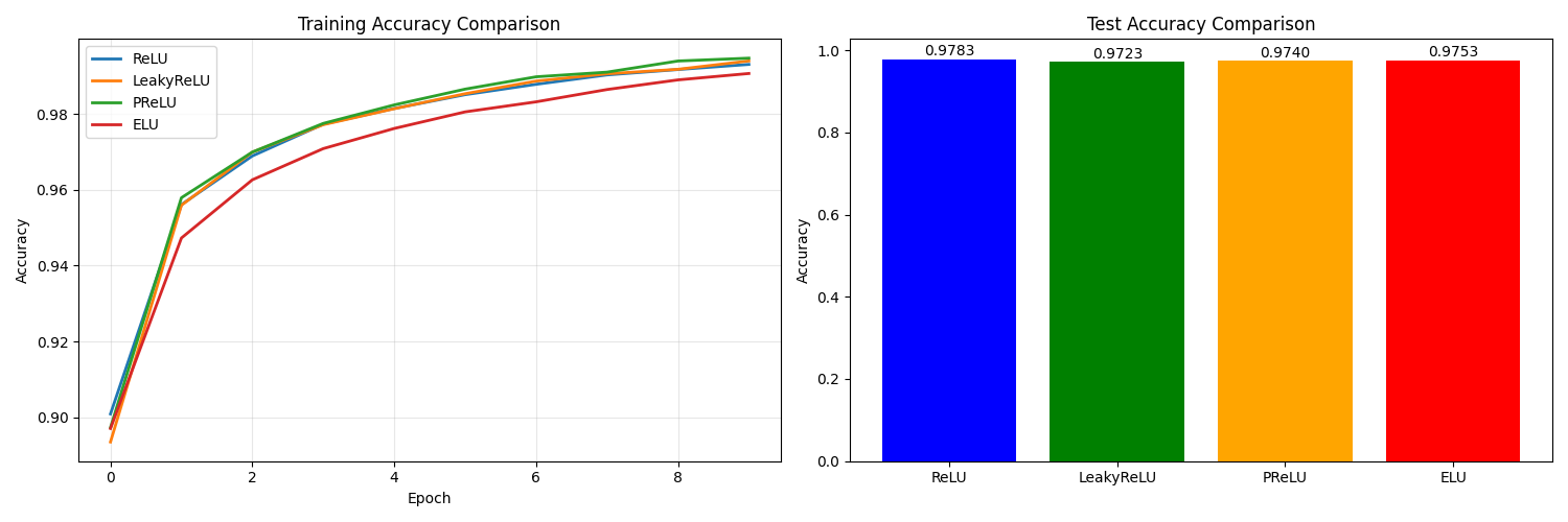
5.3 完整训练示例
import tensorflow as tf
import matplotlib.pyplot as plt

def train_with_relu_comparison():
    """比较不同ReLU变种的训练效果"""

    # 加载数据
    (x_train, y_train), (x_test, y_test) = tf.keras.datasets.mnist.load_data()

    # 数据预处理
    x_train = x_train.reshape(-1, 784).astype('float32') / 255.0
    x_test = x_test.reshape(-1, 784).astype('float32') / 255.0

    # 定义不同的激活函数
    activations = {
        'ReLU': 'relu',
        'LeakyReLU': tf.keras.layers.LeakyReLU(negative_slope=0.01),
        'PReLU': tf.keras.layers.PReLU(),
        'ELU': 'elu'
    }

    results = {}

    for name, activation in activations.items():
        print(f"\n训练使用 {name} 的模型...")

        # 创建模型
        model = tf.keras.Sequential()
        model.add(tf.keras.layers.Input(shape=(784,)))
        model.add(tf.keras.layers.Dense(128))

        # 处理激活函数 - 为PReLU创建独立实例
        if name == 'PReLU':
            model.add(tf.keras.layers.PReLU())
            model.add(tf.keras.layers.Dense(64))
            model.add(tf.keras.layers.PReLU())  # 新的独立实例
        else:
            # 其他激活函数的处理方式
            if isinstance(activation, str):
                model.add(tf.keras.layers.Activation(activation))
            else:
                model.add(activation)

            model.add(tf.keras.layers.Dense(64))

            # 再次添加激活函数
            if isinstance(activation, str):
                model.add(tf.keras.layers.Activation(activation))
            else:
                model.add(activation)

        model.add(tf.keras.layers.Dense(10, activation='softmax'))

        # 编译模型
        model.compile(
            optimizer='adam',
            loss='sparse_categorical_crossentropy',
            metrics=['accuracy']
        )

        # 训练模型
        history = model.fit(
            x_train, y_train,
            batch_size=128,
            epochs=10,
            validation_split=0.2,
            verbose=0
        )

        # 评估模型
        test_loss, test_accuracy = model.evaluate(x_test, y_test, verbose=0)

        results[name] = {
            'history': history,
            'test_accuracy': test_accuracy,
            'test_loss': test_loss
        }

        print(f"{name} - 测试准确率: {test_accuracy:.4f}")

    return results

def plot_comparison_results(results):
    """绘制比较结果"""
    plt.figure(figsize=(15, 5))

    # 训练准确率
    plt.subplot(1, 2, 1)
    for name, result in results.items():
        plt.plot(result['history'].history['accuracy'],
                label=f'{name}', linewidth=2)
    plt.title('Training Accuracy Comparison')
    plt.xlabel('Epoch')
    plt.ylabel('Accuracy')
    plt.legend()
    plt.grid(True, alpha=0.3)

    # 测试准确率比较
    plt.subplot(1, 2, 2)
    names = list(results.keys())
    accuracies = [results[name]['test_accuracy'] for name in names]

    bars = plt.bar(names, accuracies, color=['blue', 'green', 'orange', 'red'])
    plt.title('Test Accuracy Comparison')
    plt.ylabel('Accuracy')

    # 在柱状图上显示数值
    for bar, accuracy in zip(bars, accuracies):
        plt.text(bar.get_x() + bar.get_width()/2, bar.get_height() + 0.001,
                f'{accuracy:.4f}', ha='center', va='bottom')

    plt.tight_layout()
    plt.show()

# 运行比较实验
results = train_with_relu_comparison()
plot_comparison_results(results)
运行结果如下:
5.4 高级应用:自定义ReLU变种
class LearnableReLU(tf.keras.layers.Layer):
    """可学习参数的ReLU变种"""

    def __init__(self, initial_alpha=0.01, **kwargs):
        super(LearnableReLU, self).__init__(**kwargs)
        self.initial_alpha = initial_alpha

    def build(self, input_shape):
        self.alpha = self.add_weight(
            name='alpha',
            shape=(1,),
            initializer=tf.constant_initializer(self.initial_alpha),
            trainable=True
        )
        super(LearnableReLU, self).build(input_shape)

    def call(self, inputs):
        positive = tf.nn.relu(inputs)
        negative = self.alpha * (inputs - tf.abs(inputs)) * 0.5
        return positive + negative

    def get_config(self):
        config = super(LearnableReLU, self).get_config()
        config.update({'initial_alpha': self.initial_alpha})
        return config

# 使用自定义LearnableReLU
def create_advanced_network():
    model = tf.keras.Sequential([
        tf.keras.layers.Dense(128, input_shape=(784,)),
        LearnableReLU(initial_alpha=0.1),
        tf.keras.layers.Dense(64),
        LearnableReLU(initial_alpha=0.1),
        tf.keras.layers.Dense(10, activation='softmax')
    ])
    return model

# 测试自定义层
def test_learnable_relu():
    layer = LearnableReLU(initial_alpha=0.1)
    test_input = tf.constant([-2.0, -1.0, 0.0, 1.0, 2.0])
    output = layer(test_input)

    print("输入:", test_input.numpy())
    print("输出:", output.numpy())
    print("可学习参数alpha:", layer.alpha.numpy())

test_learnable_relu()
6. ReLU应用场景
6.1 计算机视觉
def relu_in_cnn():
    """CNN中的ReLU应用"""
    model = tf.keras.Sequential([
        # 卷积层 + ReLU
        tf.keras.layers.Conv2D(32, (3, 3), activation='relu', input_shape=(28, 28, 1)),
        tf.keras.layers.MaxPooling2D((2, 2)),

        tf.keras.layers.Conv2D(64, (3, 3), activation='relu'),
        tf.keras.layers.MaxPooling2D((2, 2)),

        tf.keras.layers.Conv2D(64, (3, 3), activation='relu'),
        tf.keras.layers.Flatten(),

        # 全连接层 + ReLU
        tf.keras.layers.Dense(64, activation='relu'),
        tf.keras.layers.Dense(10, activation='softmax')
    ])
    return model
6.2 自然语言处理
def relu_in_nlp():
    """NLP中的ReLU应用"""
    model = tf.keras.Sequential([
        tf.keras.layers.Embedding(10000, 128, input_length=100),
        tf.keras.layers.Flatten(),
        tf.keras.layers.Dense(256, activation='relu'),
        tf.keras.layers.Dropout(0.5),
        tf.keras.layers.Dense(128, activation='relu'),
        tf.keras.layers.Dropout(0.5),
        tf.keras.layers.Dense(1, activation='sigmoid')  # 二分类
    ])
    return model
6.3 推荐系统
def relu_in_recommendation():
    """推荐系统中的ReLU应用"""
    # 用户特征输入
    user_input = tf.keras.layers.Input(shape=(100,))
    user_features = tf.keras.layers.Dense(64, activation='relu')(user_input)

    # 物品特征输入
    item_input = tf.keras.layers.Input(shape=(50,))
    item_features = tf.keras.layers.Dense(64, activation='relu')(item_input)

    # 特征交互
    concatenated = tf.keras.layers.concatenate([user_features, item_features])
    hidden = tf.keras.layers.Dense(128, activation='relu')(concatenated)
    hidden = tf.keras.layers.Dense(64, activation='relu')(hidden)

    # 输出评分
    rating = tf.keras.layers.Dense(1, activation='linear')(hidden)

    model = tf.keras.Model(inputs=[user_input, item_input], outputs=rating)
    return model
7. 实践建议与最佳实践
7.1 何时使用ReLU?
-
默认选择:大多数前馈神经网络的隐藏层
-
CNN:卷积层之后的标准选择
-
深度网络:缓解梯度消失问题
7.2 何时避免ReLU?
-
RNN:可能导致梯度爆炸
-
输出层:根据任务选择适当的激活函数
-
对死亡神经元敏感的任务:考虑使用Leaky ReLU变种
7.3 超参数调优建议
def relu_hyperparameter_tuning():
    """ReLU超参数调优示例"""

    # 学习率与ReLU的配合
    learning_rates = [0.1, 0.01, 0.001, 0.0001]

    # 权重初始化策略
    initializers = [
        'he_normal',  # ReLU专用初始化
        'he_uniform',
        'glorot_normal',
        'random_normal'
    ]

    # 批量归一化与ReLU的配合
    def create_model_with_bn(use_batch_norm=True, learning_rate=0.001):
        model = tf.keras.Sequential([
            tf.keras.layers.Dense(128, input_shape=(784,),
                                kernel_initializer='he_normal'),
            tf.keras.layers.BatchNormalization() if use_batch_norm else tf.keras.layers.Lambda(lambda x: x),
            tf.keras.layers.ReLU(),
            tf.keras.layers.Dense(64, kernel_initializer='he_normal'),
            tf.keras.layers.BatchNormalization() if use_batch_norm else tf.keras.layers.Lambda(lambda x: x),
            tf.keras.layers.ReLU(),
            tf.keras.layers.Dense(10, activation='softmax')
        ])

        model.compile(
            optimizer=tf.keras.optimizers.Adam(learning_rate=learning_rate),
            loss='sparse_categorical_crossentropy',
            metrics=['accuracy']
        )
        return model

    return create_model_with_bn
总结
ReLU激活函数因其简单性、高效性和有效性,已经成为深度学习中最常用的激活函数之一。通过理解其数学原理、优势局限性和各种变种,我们可以在实际项目中更好地应用这一重要工具。
关键要点总结:
-
原理简单:f(x) = max(0, x),计算高效
-
解决梯度消失:正区间导数为1,支持深层网络训练
-
稀疏激活:负半轴输出为0,增强模型泛化能力
-
注意死亡ReLU:合理设置学习率和初始化策略
-
灵活使用变种:根据任务需求选择合适的ReLU变体
ReLU的成功启发了更多优秀的激活函数设计,深刻影响了深度学习的发展方向。掌握ReLU及其变种,是构建高效神经网络的重要基础。


 812
812

 被折叠的 条评论
为什么被折叠?
被折叠的 条评论
为什么被折叠?
 到【灌水乐园】发言


