


目录
前言
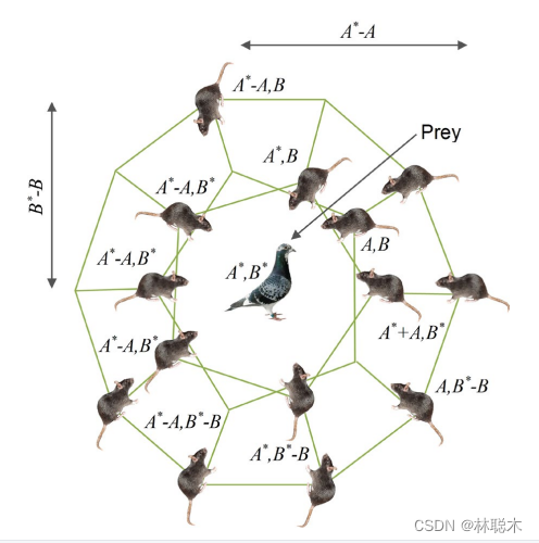
鼠群优化算法(Rat Swarm Optimizer, RSO) 是一种由Gaurav Dhiman等人在2020年提出的新型的仿生优化算法。RSO的灵感来自于自然界种鼠群追逐猎物和与猎物搏斗的行为。可以解决全局优化问题的新型仿生优化算法,它的灵感主要来自于自然界种鼠群追逐猎物和与猎物搏斗的行为。老鼠具有很丰富的社交智慧,它们通过追逐、跳跃和搏斗等各种行为相互沟通。它们具有很强的领土意识,当它们被侵犯时,就会变得非常有攻击性。
算法原理
猎物追逐
老鼠是一种社会性很强的动物,它们是通过社会群体行为来追逐猎物的。为了从数学上定义这种行为,将种群中最优个体的位置设定为猎物的位置,其他个体通过当前最优个体更新它们的位置。这个过程被定义为公式(1):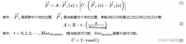
参数R随机分布在区间[1, 5],参数C随机分布在区间[0, 2]。通过调整参数A和C的取值,以在平衡算法局部搜索和全局搜索之间取得折衷。
猎物攻击
鼠群与猎物搏斗的过程可以被定义为公式(4):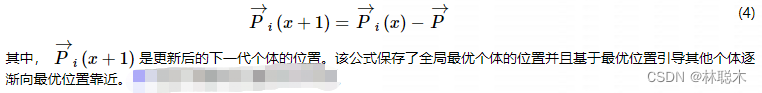
优缺点
RSO在数学上模拟了自然界种鼠群追逐猎物和与猎物搏斗的行为,并可以有效解决全局优化问题,此外它还具有结构简单和参数较少的优点。由于RSO的新颖性,关于修改或应用RSO的文献很少,但是它已经开始被应用到医药领域 。
然而,由于模拟鼠群追逐猎物的过程过于随机且不够精确,因此,RSO具有速度过慢和容易陷入局部最优等缺点。
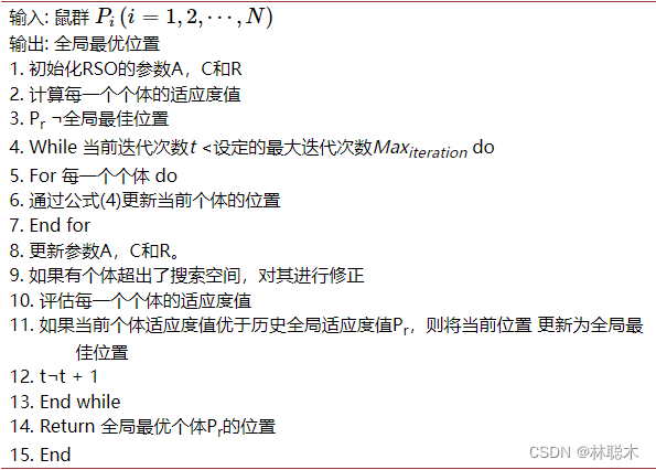
鼠群算法伪代码
算法改进
基于反向学习的DE-RSO混合优化算法,参考徐子岳,梁晓丹的论文
为了改善RSO的性能,本文提出了一种基于反向学习的DE-RSO混合优化算法(Opposition-Based Learning DE-RSO Hybrid Optimizer, OBLDE-RSO),该算法首先使用一种DE-RSO混合策略,将差分进化算法的变异机制应用到RSO中,以增加种群的多样性,然后用反向学习策略(Opposition-Based Learning, OBL),针对性地扩大个体的搜索范围,使个体以更高概率找到潜在的更加理想的求解区域。同时,为了加速算法收敛,对RSO本身的参数进行了调整优化。
DE-RSO混合策略
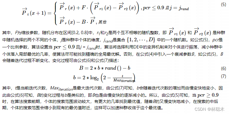
为了维持种群的多样性,将DE中的变异机制引入到RSO中,对种群中的个体进行振荡,同时在算法中引入一个参数B以提高算法的收敛速度。我们使用一个比例参数pcr来随机选择采用何种更新方式,所以鼠群搏斗的过程可以描述为公式(5):
反向学习策略
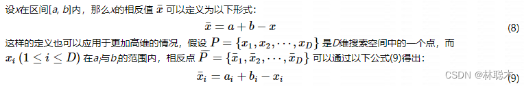
由公式(8)和公式(9)可以看出,随机的猜测点和猜测它的相反值可以同时以更高的概率来找到潜在的更加理想的求解区域,其中最优解就很有可能位于其中。
在得到一个个体的相反个体后,同时计算该个体与其相反个体的适应度值,比较两者的适应度值,若其相反个体的适应度值优于原个体的适应度值,原个体将被相反个体所替代,这样个体将会用更高的概率靠近最优个体,计算效率和计算精确度会得到明显提高
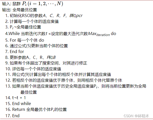
改进算法伪代码
实验结果与分析
引入了IEEE CEC2017基准测试函数集,利用该测试函数集测试OBLDE-RSO算法。IEEE CEC2017基准测试函数集由29个函数组成,包括2个单峰函数(g1, g3),7个简单多峰函数(g4-g10),10个混合函数(g11-g20)和10个组合函数(g21-g30)。 。
在本实验中,为了进行公平的比较,操作环境保持不变,如下:
1) 每个函数独立运行30次。
2) 种群规模为150,个体维度为30。
3) 函数的评估总次数为45,000次。
4) 搜索范围为[−100, 100]。
这些实验都是在一台具有I7处理器、windows 10操作系统和8 GB内存的计算机上执行的,所有算法都是在Matlab2018b中进行编码的。
为了证明OBLDE-RSO性能的优越性,我们将基于反向学习的DE-RSO混合优化算法OBLDE-RSO同鼠群算法RSO、差分进化算法DE、狮群算法LSO和遗传算法GA进行比较。
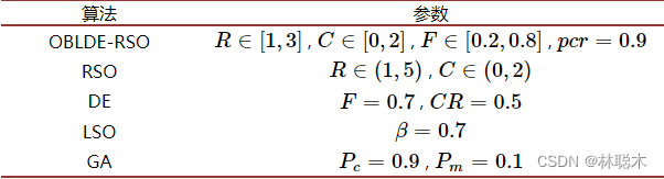
表4是OBLDE-RSO,RSO,DE,LSO和GA的对比结果,结果包括各算法在测试函数集中独立运行30次的平均值(Mean)和标准差(Std)。
表4 OBLDE-RSO,RSO,DE,LSO和GA的对比结果
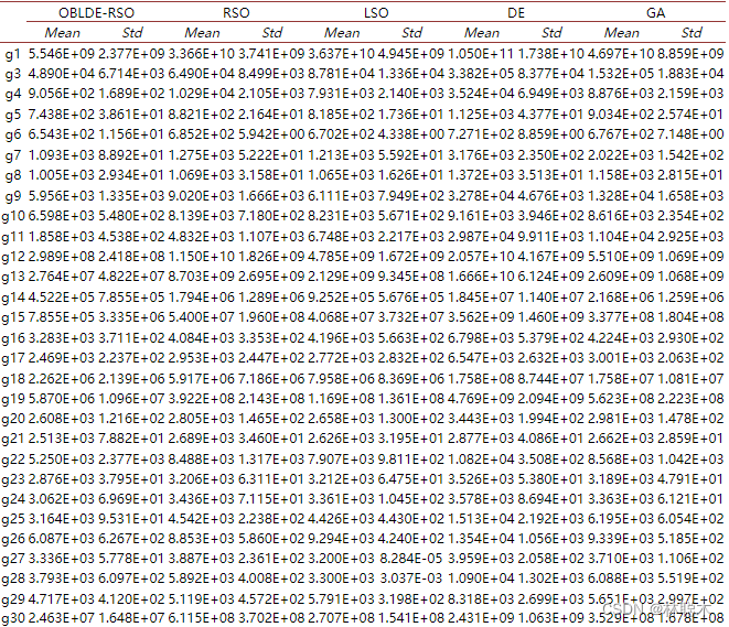
由表4可知,在大部分情况下OBLDE-RSO的性能优于RSO、DE、LSO、GA。具体来说,在29个测试函数中,OBLDE-RSO在其中的27个对RSO、DE、LSO、GA表现出了更加出色的性能。OBLDE-RSO在单峰函数、简单多峰函数和混合函数上,在求解的精确度上比其他比较算法具有绝对的优势。在组合函数上,OBLDE-RSO也具有十分优异的性能。这说明DE-RSO混合策略和反向学习策略的使用也可以提高RSO的性能。
另外,在四类测试函数中各挑取一个代表函数(g1, g6, g16, g24)绘制收敛图和盒型图,以进一步分析实验结果。图1和图2分别是算法在四个函数中的测试后的收敛图和盒型图。
图1中可以直观地展示出OBLDE-RSO,RSO,LSO,DE和GA的收敛性能。OBLDE-RSO的收敛趋势线比其他比较算法的收敛速度更快,同时,OBLDE-RSO的收敛精度也高于其他比较算法,这进一步证实了使用两种策略可以提高算法的收敛速度和收敛精度。
在图2中,盒型图展示出4次实验得到的实验结果。由图可以看出,在绝大多数情况下,OBLDE-RSO的结果优于其他比较算法,说明OBLDE-RSO具有更加优越和稳定的数据结构。
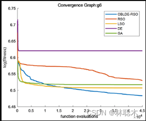
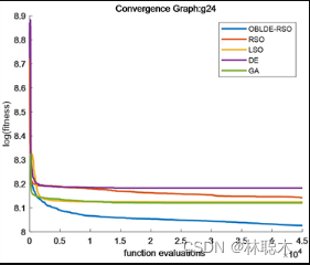
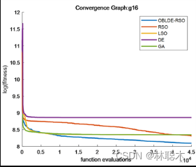
图1 各算法的收敛曲线对比图

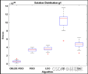
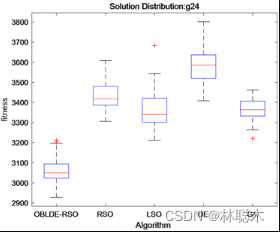
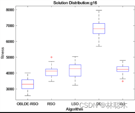
图2 算法的盒图对比结果
结论
基于反向学习的DE-RSO混合优化算法,算法使用了DE-RSO混合策略和反向学习策略以提高算法的性能。DE-RSO混合策略使用变异机制以保持种群多样性并降低算法陷入局部最优的可能性,可以有效改善RSO过早收敛的缺点。OBL策略可以针对性地扩大个体的搜索范围,使个体以更高概率找到潜在的更加理想的求解区域。同时添加一个参数B以控制算法在搜索前期和后期的不同搜索任务。通过对比OBLDE-RSO和其它比较算法在IEEE CEC2017测试函数集上的实验数据和图像,证明了使用了两种策略后,算法的局部搜索能力和全局搜索能力都得到了很大的提升。
代码
MATLAB
fun_info
-
function [lowerbound,upperbound,dimension,fitness]
= fun_info(F)
-
-
-
switch F
-
case
'F1'
-
fitness
= @F
1;
-
lowerbound
=-
100;
-
upperbound
=
100;
-
dimension
=
30;
-
-
case
'F2'
-
fitness
= @F
2;
-
lowerbound
=-
10;
-
upperbound
=
10;
-
dimension
=
30;
-
-
case
'F3'
-
fitness
= @F
3;
-
lowerbound
=-
100;
-
upperbound
=
100;
-
dimension
=
30;
-
-
case
'F4'
-
fitness
= @F
4;
-
lowerbound
=-
100;
-
upperbound
=
100;
-
dimension
=
30;
-
-
case
'F5'
-
fitness
= @F
5;
-
lowerbound
=-
30;
-
upperbound
=
30;
-
dimension
=
30;
-
-
case
'F6'
-
fitness
= @F
6;
-
lowerbound
=-
100;
-
upperbound
=
100;
-
dimension
=
30;
-
-
case
'F7'
-
fitness
= @F
7;
-
lowerbound
=-
1.28;
-
upperbound
=
1.28;
-
dimension
=
30;
-
-
case
'F8'
-
fitness
= @F
8;
-
lowerbound
=-
500;
-
upperbound
=
500;
-
dimension
=
30;
-
-
case
'F9'
-
fitness
= @F
9;
-
lowerbound
=-
5.12;
-
upperbound
=
5.12;
-
dimension
=
30;
-
-
case
'F10'
-
fitness
= @F
10;
-
lowerbound
=-
32;
-
upperbound
=
32;
-
dimension
=
30;
-
-
case
'F11'
-
fitness
= @F
11;
-
lowerbound
=-
600;
-
upperbound
=
600;
-
dimension
=
30;
-
-
case
'F12'
-
fitness
= @F
12;
-
lowerbound
=-
50;
-
upperbound
=
50;
-
dimension
=
30;
-
-
case
'F13'
-
fitness
= @F
13;
-
lowerbound
=-
50;
-
upperbound
=
50;
-
dimension
=
30;
-
-
case
'F14'
-
fitness
= @F
14;
-
lowerbound
=-
65.536;
-
upperbound
=
65.536;
-
dimension
=
2;
-
-
case
'F15'
-
fitness
= @F
15;
-
lowerbound
=-
5;
-
upperbound
=
5;
-
dimension
=
4;
-
-
case
'F16'
-
fitness
= @F
16;
-
lowerbound
=-
5;
-
upperbound
=
5;
-
dimension
=
2;
-
-
case
'F17'
-
fitness
= @F
17;
-
lowerbound
=[-
5,0];
-
upperbound
=[
10,15];
-
dimension
=
2;
-
-
case
'F18'
-
fitness
= @F
18;
-
lowerbound
=-
2;
-
upperbound
=
2;
-
dimension
=
2;
-
-
case
'F19'
-
fitness
= @F
19;
-
lowerbound
=
0;
-
upperbound
=
1;
-
dimension
=
3;
-
-
case
'F20'
-
fitness
= @F
20;
-
lowerbound
=
0;
-
upperbound
=
1;
-
dimension
=
6;
-
-
case
'F21'
-
fitness
= @F
21;
-
lowerbound
=
0;
-
upperbound
=
10;
-
dimension
=
4;
-
-
case
'F22'
-
fitness
= @F
22;
-
lowerbound
=
0;
-
upperbound
=
10;
-
dimension
=
4;
-
-
case
'F23'
-
fitness
= @F
23;
-
lowerbound
=
0;
-
upperbound
=
10;
-
dimension
=
4;
-
end
-
-
end
-
-
% F
1
-
-
function R
= F
1(x)
-
R
=
sum(x.^
2);
-
end
-
-
% F
2
-
-
function R
= F
2(x)
-
R
=
sum(abs(x))
+prod(abs(x));
-
end
-
-
% F
3
-
-
function R
= F
3(x)
-
dimension
=
size(x,
2);
-
R
=
0;
-
for i
=
1:dimension
-
R
=R
+
sum(x(
1:i))^
2;
-
end
-
end
-
-
% F
4
-
-
function R
= F
4(x)
-
R
=max(abs(x));
-
end
-
-
% F
5
-
-
function R
= F
5(x)
-
dimension
=
size(x,
2);
-
R
=
sum(
100
*(x(
2:dimension)-(x(
1:dimension-
1).^
2)).^
2
+(x(
1:dimension-
1)-
1).^
2);
-
end
-
-
% F
6
-
-
function R
= F
6(x)
-
R
=
sum(abs((x
+.
5)).^
2);
-
end
-
-
% F
7
-
-
function R
= F
7(x)
-
dimension
=
size(x,
2);
-
R
=
sum([
1:dimension].
*(x.^
4))
+rand;
-
end
-
-
% F
8
-
-
function R
= F
8(x)
-
R
=
sum(-x.
*sin(sqrt(abs(x))));
-
end
-
-
% F
9
-
-
function R
= F
9(x)
-
dimension
=
size(x,
2);
-
R
=
sum(x.^
2-
10
*cos(
2
*pi.
*x))
+
10
*dimension;
-
end
-
-
% F
10
-
-
function R
= F
10(x)
-
dimension
=
size(x,
2);
-
R
=-
20
*exp(-.
2
*sqrt(
sum(x.^
2)
/dimension))-exp(
sum(cos(
2
*pi.
*x))
/dimension)
+
20
+exp(
1);
-
end
-
-
% F
11
-
-
function R
= F
11(x)
-
dimension
=
size(x,
2);
-
R
=
sum(x.^
2)
/
4000-prod(cos(x.
/sqrt([
1:dimension])))
+
1;
-
end
-
-
% F
12
-
-
function R
= F
12(x)
-
dimension
=
size(x,
2);
-
R
=(pi
/dimension)
*(
10
*((sin(pi
*(
1
+(
x(1)
+
1)
/
4)))^
2)
+
sum((((x(
1:dimension-
1)
+
1).
/
4).^
2).
*...
-
(
1
+
10.
*((sin(pi.
*(
1
+(x(
2:dimension)
+
1).
/
4)))).^
2))
+((x(dimension)
+
1)
/
4)^
2)
+
sum(Ufun(x,
10,100,4));
-
end
-
-
% F
13
-
-
function R
= F
13(x)
-
dimension
=
size(x,
2);
-
R
=.
1
*((sin(
3
*pi
*
x(1)))^
2
+
sum((x(
1:dimension-
1)-
1).^
2.
*(
1
+(sin(
3.
*pi.
*x(
2:dimension))).^
2))
+...
-
((x(dimension)-
1)^
2)
*(
1
+(sin(
2
*pi
*x(dimension)))^
2))
+
sum(Ufun(x,
5,100,4));
-
end
-
-
% F
14
-
-
function R
= F
14(x)
-
aS
=[-
32 -
16
0
16
32 -
32 -
16
0
16
32 -
32 -
16
0
16
32 -
32 -
16
0
16
32 -
32 -
16
0
16
32;,...
-
-
32 -
32 -
32 -
32 -
32 -
16 -
16 -
16 -
16 -
16
0
0
0
0
0
16
16
16
16
16
32
32
32
32
32];
-
-
for j
=
1:
25
-
bS(j)
=
sum((x
'-aS(:,j)).^6);
-
end
-
R=(1/500+sum(1./([1:25]+bS))).^(-1);
-
end
-
-
% F15
-
-
function R = F15(x)
-
aK=[.1957 .1947 .1735 .16 .0844 .0627 .0456 .0342 .0323 .0235 .0246];
-
bK=[.25 .5 1 2 4 6 8 10 12 14 16];bK=1./bK;
-
R=sum((aK-((x(1).*(bK.^2+x(2).*bK))./(bK.^2+x(3).*bK+x(4)))).^2);
-
end
-
-
% F16
-
-
function R = F16(x)
-
R=4*(x(1)^2)-2.1*(x(1)^4)+(x(1)^6)/3+x(1)*x(2)-4*(x(2)^2)+4*(x(2)^4);
-
end
-
-
% F17
-
-
function R = F17(x)
-
R=(x(2)-(x(1)^2)*5.1/(4*(pi^2))+5/pi*x(1)-6)^2+10*(1-1/(8*pi))*cos(x(1))+10;
-
end
-
-
% F18
-
-
function R = F18(x)
-
R=(1+(x(1)+x(2)+1)^2*(19-14*x(1)+3*(x(1)^2)-14*x(2)+6*x(1)*x(2)+3*x(2)^2))*...
-
(30+(2*x(1)-3*x(2))^2*(18-32*x(1)+12*(x(1)^2)+48*x(2)-36*x(1)*x(2)+27*(x(2)^2)));
-
end
-
-
% F19
-
-
function R = F19(x)
-
aH=[3 10 30;.1 10 35;3 10 30;.1 10 35];cH=[1 1.2 3 3.2];
-
pH=[.3689 .117 .2673;.4699 .4387 .747;.1091 .8732 .5547;.03815 .5743 .8828];
-
R=0;
-
for i=1:4
-
R=R-cH(i)*exp(-(sum(aH(i,:).*((x-pH(i,:)).^2))));
-
end
-
end
-
-
% F20
-
-
function R = F20(x)
-
aH=[10 3 17 3.5 1.7 8;.05 10 17 .1 8 14;3 3.5 1.7 10 17 8;17 8 .05 10 .1 14];
-
cH=[1 1.2 3 3.2];
-
pH=[.1312 .1696 .5569 .0124 .8283 .5886;.2329 .4135 .8307 .3736 .1004 .9991;...
-
.2348 .1415 .3522 .2883 .3047 .6650;.4047 .8828 .8732 .5743 .1091 .0381];
-
R=0;
-
for i=1:4
-
R=R-cH(i)*exp(-(sum(aH(i,:).*((x-pH(i,:)).^2))));
-
end
-
end
-
-
% F21
-
-
function R = F21(x)
-
aSH=[4 4 4 4;1 1 1 1;8 8 8 8;6 6 6 6;3 7 3 7;2 9 2 9;5 5 3 3;8 1 8 1;6 2 6 2;7 3.6 7 3.6];
-
cSH=[.1 .2 .2 .4 .4 .6 .3 .7 .5 .5];
-
-
R=0;
-
for i=1:5
-
R=R-((x-aSH(i,:))*(x-aSH(i,:))'
+cSH(i))^(-
1);
-
end
-
end
-
-
% F
22
-
-
function R
= F
22(x)
-
aSH
=[
4
4
4
4;
1
1
1
1;
8
8
8
8;
6
6
6
6;
3
7
3
7;
2
9
2
9;
5
5
3
3;
8
1
8
1;
6
2
6
2;
7
3.6
7
3.6];
-
cSH
=[.
1 .
2 .
2 .
4 .
4 .
6 .
3 .
7 .
5 .
5];
-
-
R
=
0;
-
for i
=
1:
7
-
R
=R-((x-aSH(i,:))
*(x-aSH(i,:))
'+cSH(i))^(-1);
-
end
-
end
-
-
% F23
-
-
function R = F23(x)
-
aSH=[4 4 4 4;1 1 1 1;8 8 8 8;6 6 6 6;3 7 3 7;2 9 2 9;5 5 3 3;8 1 8 1;6 2 6 2;7 3.6 7 3.6];
-
cSH=[.1 .2 .2 .4 .4 .6 .3 .7 .5 .5];
-
-
R=0;
-
for i=1:10
-
R=R-((x-aSH(i,:))*(x-aSH(i,:))'
+cSH(i))^(-
1);
-
end
-
end
-
-
function R
=Ufun(x,a,k,m)
-
R
=k.
*((x-a).^m).
*(x
>a)
+k.
*((-x-a).^m).
*(x
<(-a));
-
end

fun_plot
-
function fun_plot(fun_name)
-
-
[lowerbound,upperbound,dimension,fitness]
=fun_info(fun_name);
-
-
switch fun_name
-
case
'F1'
-
x
=-
100:
2:
100; y
=x; %[-
100,100]
-
-
case
'F2'
-
x
=-
100:
2:
100; y
=x; %[-
10,10]
-
-
case
'F3'
-
x
=-
100:
2:
100; y
=x; %[-
100,100]
-
-
case
'F4'
-
x
=-
100:
2:
100; y
=x; %[-
100,100]
-
case
'F5'
-
x
=-
200:
2:
200; y
=x; %[-
5,5]
-
case
'F6'
-
x
=-
100:
2:
100; y
=x; %[-
100,100]
-
case
'F7'
-
x
=-
1:
0.03:
1; y
=x %[-
1,1]
-
case
'F8'
-
x
=-
500:
10:
500;y
=x; %[-
500,500]
-
case
'F9'
-
x
=-
5:
0.1:
5; y
=x; %[-
5,5]
-
case
'F10'
-
x
=-
20:
0.5:
20; y
=x;%[-
500,500]
-
case
'F11'
-
x
=-
500:
10:
500; y
=x;%[-
0.5,0.5]
-
case
'F12'
-
x
=-
10:
0.1:
10; y
=x;%[-pi,pi]
-
case
'F13'
-
x
=-
5:
0.08:
5; y
=x;%[-
3,1]
-
case
'F14'
-
x
=-
100:
2:
100; y
=x;%[-
100,100]
-
case
'F15'
-
x
=-
5:
0.1:
5; y
=x;%[-
5,5]
-
case
'F16'
-
x
=-
1:
0.01:
1; y
=x;%[-
5,5]
-
case
'F17'
-
x
=-
5:
0.1:
5; y
=x;%[-
5,5]
-
case
'F18'
-
x
=-
5:
0.06:
5; y
=x;%[-
5,5]
-
case
'F19'
-
x
=-
5:
0.1:
5; y
=x;%[-
5,5]
-
case
'F20'
-
x
=-
5:
0.1:
5; y
=x;%[-
5,5]
-
case
'F21'
-
x
=-
5:
0.1:
5; y
=x;%[-
5,5]
-
case
'F22'
-
x
=-
5:
0.1:
5; y
=x;%[-
5,5]
-
case
'F23'
-
x
=-
5:
0.1:
5; y
=x;%[-
5,5]
-
end
-
-
-
-
L
=
length(x);
-
f
=[];
-
-
for i
=
1:L
-
for j
=
1:L
-
if strcmp(fun_name,
'F15')
=
=
0
&
& strcmp(fun_name,
'F19')
=
=
0
&
& strcmp(fun_name,
'F20')
=
=
0
&
& strcmp(fun_name,
'F21')
=
=
0
&
& strcmp(fun_name,
'F22')
=
=
0
&
& strcmp(fun_name,
'F23')
=
=
0
-
f(i,j)
=fitness([x(i),y(j)]);
-
end
-
if strcmp(fun_name,
'F15')
=
=
1
-
f(i,j)
=fitness([x(i),y(j),
0,0]);
-
end
-
if strcmp(fun_name,
'F19')
=
=
1
-
f(i,j)
=fitness([x(i),y(j),
0]);
-
end
-
if strcmp(fun_name,
'F20')
=
=
1
-
f(i,j)
=fitness([x(i),y(j),
0,0,0,0]);
-
end
-
if strcmp(fun_name,
'F21')
=
=
1 || strcmp(fun_name,
'F22')
=
=
1 ||strcmp(fun_name,
'F23')
=
=
1
-
f(i,j)
=fitness([x(i),y(j),
0,0]);
-
end
-
end
-
end
-
-
surfc(x,y,f,
'LineStyle',
'none');
-
-
end
-
init
-
function Pos
=init(SearchAgents,dimension,upperbound,lowerbound)
-
-
Boundary
=
size(upperbound,
2);
-
if Boundary
=
=
1
-
Pos
=rand(SearchAgents,dimension).
*(upperbound-lowerbound)
+lowerbound;
-
end
-
-
if Boundary
>
1
-
for i
=
1:dimension
-
ub_i
=upperbound(i);
-
lb_i
=lowerbound(i);
-
Pos(:,i)
=rand(SearchAgents,
1).
*(ub_i-lb_i)
+lb_i;
-
end
-
end
main
-
% Published paper: G. Dhiman et al. %
-
% A novel algorithm
for
global optimization: Rat Swarm Optimizer %
-
% Jounral
of Ambient Intelligence
and Humanized Computing %
-
% DOI: https:
/
/doi.org
/
10.1007
/s
12652-
020-
02580-
0 %
-
clear
all
-
clc
-
SearchAgents
=
30;
-
Fun_name
=
'F1';
-
Max_iterations
=
1000;
-
[lowerbound,upperbound,dimension,fitness]
=fun_info(Fun_name);
-
[Best_score,Best_pos,SHO_curve]
=rso(SearchAgents,Max_iterations,lowerbound,upperbound,dimension,fitness);
-
-
figure(
'Position',[
500
500
660
290])
-
%Draw
search
space
-
subplot(
1,2,1);
-
fun_plot(Fun_name);
-
title(
'Parameter space')
-
xlabel(
'x_1');
-
ylabel(
'x_2');
-
zlabel([Fun_name,
'( x_1 , x_2 )'])
-
-
%Draw objective
space
-
subplot(
1,2,2);
-
plots
=semilogy(SHO_curve,
'Color',
'g');
-
set(plots,
'linewidth',
2)
-
title(
'Objective space')
-
xlabel(
'Iterations');
-
ylabel(
'Best score');
-
-
axis tight
-
grid
on
-
box
on
-
-
legend(
'RSO')
-
-
display([
'The best optimal value of the objective function found by RSO is : ', num
2str(Best_score)]);
-
-
-
-
-
RSO
-
function[Score,Position,Convergence]
=rso(
Search_Agents,Max_iterations,Lower_bound,Upper_bound,dimension,objective)
-
Position
=
zeros(
1,dimension);
-
Score
=inf;
-
Positions
=init(
Search_Agents,dimension,Upper_bound,Lower_bound);
-
Convergence
=
zeros(
1,Max_iterations);
-
l
=
0;
-
x
=
1;
-
y
=
5;
-
R
= floor((y-x).
*rand(
1,1)
+ x);
-
while l
<Max_iterations
-
for i
=
1:
size(Positions,
1)
-
-
Flag
4Upper_bound
=Positions(i,:)
>Upper_bound;
-
Flag
4Lower_bound
=Positions(i,:)
<Lower_bound;
-
Positions(i,:)
=(Positions(i,:).
*(~(Flag
4Upper_bound
+Flag
4Lower_bound)))
+Upper_bound.
*Flag
4Upper_bound
+Lower_bound.
*Flag
4Lower_bound;
-
-
fitness
=objective(Positions(i,:));
-
-
if fitness
<Score
-
Score
=fitness;
-
Position
=Positions(i,:);
-
end
-
-
end
-
-
A
=R-l
*((R)
/Max_iterations);
-
-
for i
=
1:
size(Positions,
1)
-
for j
=
1:
size(Positions,
2)
-
C
=
2
*rand();
-
P_vec
=A
*Positions(i,j)
+abs(C
*((Position(j)-Positions(i,j))));
-
P_
final
=Position(j)-P_vec;
-
Positions(i,j)
=P_
final;
-
-
end
-
end
-
l
=l
+
1;
-
Convergence(l)
=Score;
-
end


 1719
1719


 被折叠的 条评论
为什么被折叠?
被折叠的 条评论
为什么被折叠?
 到【灌水乐园】发言


