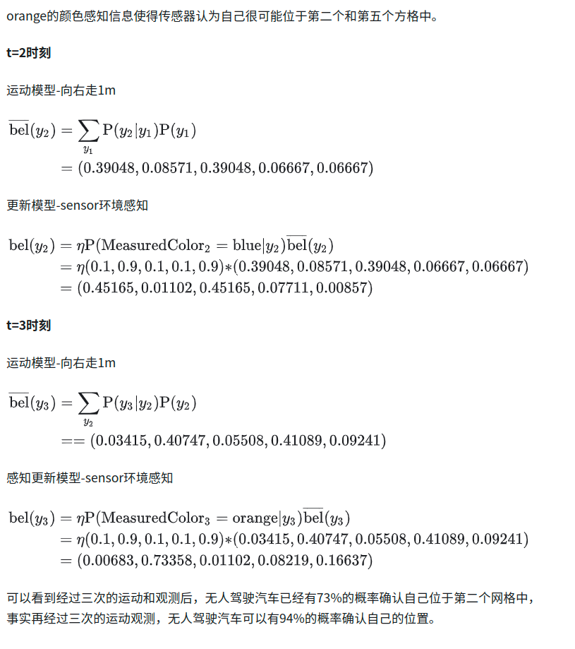
自动驾驶定位算法-直方图滤波(Histogram Filter)定位

adsdriver

于 2024-04-10 20:46:49 发布

阅读量410

点赞数 10

文章标签：自动驾驶定位算法直方图滤波

本文链接：https://blog.csdn.net/liuphahaha/article/details/137610382

版权

自动驾驶定位算法-直方图滤波(Histogram Filter)定位

附赠自动驾驶学习资料和量产经验：链接

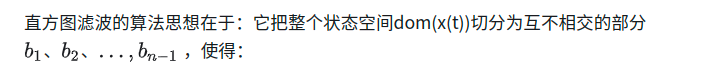
1、直方图滤波(Histogram Filter)的算法思想

2、1D直方图滤波在自动驾驶定位的应用

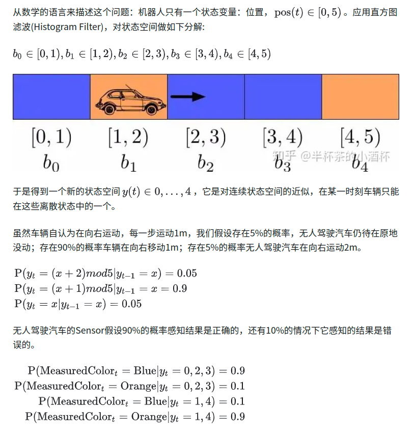
如下图所示，无人驾驶汽车在一维的宽度为5m的世界重复循环，因为世界是循环的，所以如果无人驾驶汽车到了最右侧，再往前走一步，它就又回到了最左侧的位置。

自动驾驶汽车上安装有Sensor可以检测车辆当前所在位置的颜色，但Sensor本身的存在一定检测错误率，即Sensor对颜色的检测不是100%准确的；

无人驾驶汽车以自认为1m/step的恒定速度向右运动，车辆运动本身也存在误差，即向车辆发出的控制命令是向右移动2m，而实际的车辆运动结果可能是待在原地不动，可能向右移动1m，也可能向右移动3m。

2.1 数学模型

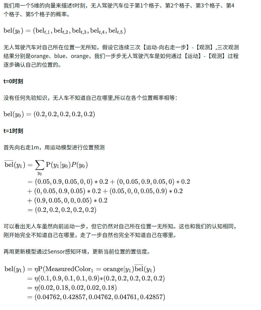
2.2 利用直方图滤波(Histogram Filter)进行车辆定位的过程

3、2D直方图滤波在自动驾驶定位中的应用(一)

1D的直方图滤波可以很好的帮助我们理解直方图滤波的原理以及在如何应用在自动驾驶的定位过程中。但是1D的直方图滤波在实际应用中几乎是不存在的，所以我们从更偏向应用的角度，看看2D直方图滤波在自动驾驶定位中是如何工作的。

3.1 定义二维地图

首先定义一张二维地图，R和G代表地图块的颜色：R为红色，G为绿色。每个地图块的大小根据实际应用而定，比如0.0125m*0.125m、0.025m*0.025m等。地图块越小，定位精度越高，但是地图数据量和计算量也就越大；反之，地图块越大，定位精度越低，但数据量和计算量也相应较低。

grid = [
    [R,G,G,G,R,R,R],
    [G,G,R,G,R,G,R],
    [G,R,G,G,G,G,R],
    [R,R,G,R,G,G,G],
    [R,G,R,G,R,R,R],
    [G,R,R,R,G,R,G],
    [R,R,R,G,R,G,G],
]

t=0时刻，车辆不知道自己处于地图中的具体位置，转化为数学表述，就是车辆在各个地图块的置信度相同，代码如下:

def initialize_beliefs(grid):
    height = len(grid)
    width = len(grid[0])
    area = height * width
    belief_per_cell = 1.0 / area
    beliefs = []
    for i in range(height):
        row = []
        for j in range(width):
            row.append(belief_per_cell)
        beliefs.append(row)
    return beliefs

初始置信度如下:

0.020  0.020  0.020  0.020  0.020  0.020  0.020  
0.020  0.020  0.020  0.020  0.020  0.020  0.020  
0.020  0.020  0.020  0.020  0.020  0.020  0.020  
0.020  0.020  0.020  0.020  0.020  0.020  0.020  
0.020  0.020  0.020  0.020  0.020  0.020  0.020  
0.020  0.020  0.020  0.020  0.020  0.020  0.020  
0.020  0.020  0.020  0.020  0.020  0.020  0.020

置信度的可视化如下，红色星星位置为车辆的真实初始实际位置，蓝色圈大小代表置信度的高低，蓝色圈越大，置信度越高，蓝色圈越小，置信度越低。t=0时刻，车辆不确定自己的位置，所以各个位置的置信度相等。

3.2 运动更新

车辆运动模型简化为x、y两个方向的运动，同时由于运动的不确定性，需要对运动后的位置增加概率性信息。

代码如下:

def move(dy, dx, beliefs, blurring):
    height = len(beliefs)
    width = len(beliefs[0])
    new_G = [[0.0 for i in range(width)] for j in range(height)]
    for i, row in enumerate(beliefs):
        for j, cell in enumerate(row):
            new_i = (i + dy ) % height
            new_j = (j + dx ) % width
            new_G[int(new_i)][int(new_j)] = cell
    return blur(new_G, blurring)

3.3 观测更新

观测更新的过程中，当观测的Color等于地图块的Color时，hit=1， bel=beliefs[i][j] * p_hit；当观测到的Color不等于地图块的Color时，hit=0， bel=beliefs[i][j] * p_miss。

代码如下:

def sense(color, grid, beliefs, p_hit, p_miss):
    new_beliefs = []
 
    height = len(grid)
    width = len(grid[0])
    
    # loop through all grid cells
    for i in range(height):
        row = []
        for j in range(width):
            hit = (color == grid[i][j])
            row.append(beliefs[i][j] * (hit * p_hit + (1-hit) * p_miss))
        new_beliefs.append(row)
        
    s = sum(map(sum, new_beliefs))

    for i in range(height):
        for j in range(width):
            new_beliefs[i][j] = new_beliefs[i][j] / s
            
    return new_beliefs

3.4 运行定位流程

单次直方图滤波定位过程中，先进行观测更新，再进行运动更新。

def run(self, num_steps=1):
    for i in range(num_steps):
	self.sense()
	dy, dx = self.random_move()
	self.move(dy,dx)

设置运动更新的不确定度为0.1，观测更新的错误率：每隔100次观测出现一次观测错误，车辆的真实初始位置为(3,3),注意，这个真实位置车辆自己并不知道，我们只是为了仿真而设置的值。

blur = 0.1
p_hit = 100.0
init_pos = (3,3)
simulation = sim.Simulation(grid, blur, p_hit, init_pos)

simulation.run(1)
simulation.show_beliefs()
show_rounded_beliefs(simulation.beliefs)

经过一次直方图滤波定位之后，各个位置的置信度已经发生了变化。

0.003  0.002  0.036  0.002  0.037  0.003  0.038  
0.003  0.037  0.002  0.002  0.001  0.002  0.037  
0.038  0.038  0.003  0.036  0.002  0.002  0.003  
0.038  0.004  0.038  0.003  0.037  0.038  0.038  
0.003  0.038  0.039  0.038  0.003  0.037  0.003  
0.038  0.038  0.038  0.003  0.037  0.003  0.003  
0.038  0.003  0.002  0.002  0.038  0.038  0.038

置信度的可视化效果如下。可以看到，车辆已经对自己的置信度有了一定的认知，但是还是有大量的可能位置需要进一步确认。

连续执行直方图滤波100次，各个位置置信度的数值如下:

0.008  0.000  0.000  0.000  0.000  0.016  0.016  
0.032  0.001  0.000  0.000  0.001  0.032  0.833  
0.016  0.000  0.000  0.000  0.000  0.025  0.017  
0.001  0.000  0.000  0.000  0.000  0.000  0.000  
0.000  0.000  0.000  0.000  0.000  0.000  0.000  
0.000  0.000  0.000  0.000  0.000  0.000  0.000  
0.000  0.000  0.000  0.000  0.000  0.000  0.000

置信度的可视化效果如下,可以看到，车辆已经83.3%的概率可以确定自己所处的位置了。

4、2D直方图滤波在自动驾驶定位中的应用(二)

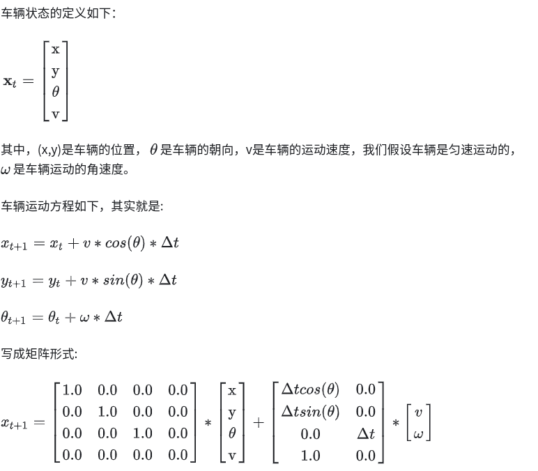
车辆的运动模型代码如下:

def motion_model(x, u):
    F = np.array([[1.0, 0, 0, 0],
                  [0, 1.0, 0, 0],
                  [0, 0, 1.0, 0],
                  [0, 0, 0, 0]])

    B = np.array([[DT * math.cos(x[2, 0]), 0],
                  [DT * math.sin(x[2, 0]), 0],
                  [0.0, DT],
                  [1.0, 0.0]])

    x = F @ x + B @ u

    return x

4.1 运动更新

运动更新的过程与前面谈到的车辆运动模型一致，车辆运动有不确定性，所以增加了Gaussian Filter用来处理不确定性。还有一个细节，就是车辆运动距离和直方图滤波的分块地图之间的转换关系：

x_shift = Δ x / map_x_resolution

y_shift = Δ y / map_y_resolution

代码如下:

# grid_map是网格地图，u=(v,w)是车辆运动的控制参数，yaw是车辆朝向
def motion_update(grid_map, u, yaw):
    # DT是时间间隔
    grid_map.dx += DT * math.cos(yaw) * u[0]
    grid_map.dy += DT * math.sin(yaw) * u[0]
    # grid_map.xy_reso是地图分辨率
    x_shift = grid_map.dx // grid_map.xy_reso
    y_shift = grid_map.dy // grid_map.xy_reso

    if abs(x_shift) >= 1.0 or abs(y_shift) >= 1.0:  # map should be shifted
        grid_map = map_shift(grid_map, int(x_shift), int(y_shift))
        grid_map.dx -= x_shift * grid_map.xy_reso
        grid_map.dy -= y_shift * grid_map.xy_reso
    # MOTION_STD是车辆运动不确定性的标准差
    grid_map.data = gaussian_filter(grid_map.data, sigma=MOTION_STD)

    return grid_map

4.2 观测更新

这个例子中通过测量车辆到LandMark的距离来确定自身的位置，LandMark的位置都是已知的。

def calc_gaussian_observation_pdf(gmap, z, iz, ix, iy, std):
    # predicted range
    x = ix * gmap.xy_reso + gmap.minx
    y = iy * gmap.xy_reso + gmap.miny
    d = math.sqrt((x - z[iz, 1]) ** 2 + (y - z[iz, 2]) ** 2)

    # likelihood
    pdf = (1.0 - norm.cdf(abs(d - z[iz, 0]), 0.0, std))

    return pdf

    #z=[(车辆到Landmark的测量距离，Landmark的x坐标，Landmark的y坐标),...]，z是所有Landmark测量距离和位置的集合，std是测量误差的标准差
def observation_update(gmap, z, std):
    for iz in range(z.shape[0]):
        for ix in range(gmap.xw):
            for iy in range(gmap.yw):
                gmap.data[ix][iy] *= calc_gaussian_observation_pdf(
                    gmap, z, iz, ix, iy, std)

    # 概率归一化
    gmap = normalize_probability(gmap)

    return gmap

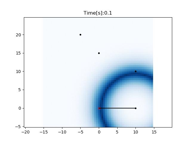
4.3 运行定位流程

设置地图和测量相关参数:

DT = 0.1  # time tick [s]
MAX_RANGE = 10.0  # maximum observation range
MOTION_STD = 1.0  # standard deviation for motion gaussian distribution
RANGE_STD = 3.0  # standard deviation for observation gaussian distribution

# grid map param
XY_RESO = 0.5  # xy grid resolution
MINX = -15.0
MINY = -5.0
MAXX = 15.0
MAXY = 25.0

# Landmark Position
RF_ID = np.array([[10.0, 0.0],
                 [10.0, 10.0],
                 [0.0, 15.0],
                 [-5.0, 20.0]])
# 车辆的初始位置(for simulation)
xTrue = np.zeros((4, 1))

通过Observation模拟自动驾驶车辆对各个LandMark的观测结果和车辆速度的误差。

def observation(xTrue, u, RFID):
    xTrue = motion_model(xTrue, u)

    z = np.zeros((0, 3))

    for i in range(len(RFID[:, 0])):

        dx = xTrue[0, 0] - RFID[i, 0]
        dy = xTrue[1, 0] - RFID[i, 1]
        d = math.sqrt(dx ** 2 + dy ** 2)
        if d <= MAX_RANGE:
            # add noise to range observation
            dn = d + np.random.randn() * NOISE_RANGE
            zi = np.array([dn, RFID[i, 0], RFID[i, 1]])
            z = np.vstack((z, zi))

    # add noise to speed
    ud = u[:, :]
    ud[0] += np.random.randn() * NOISE_SPEED

    return xTrue, z, ud

执行车辆定位流程:

    while SIM_TIME >= time:
        time += DT
        print("Time:", time)

        u = calc_input()

        yaw = xTrue[2, 0]  # Orientation is known
        xTrue, z, ud = observation(xTrue, u, RF_ID)

        grid_map = histogram_filter_localization(grid_map, u, z, yaw)

定位效果如下:

adsdriver

关注

10
点赞
踩
10

收藏

觉得还不错? 一键收藏
0
评论
自动驾驶定位算法-直方图滤波(Histogram Filter)定位

首先定义一张二维地图，R和G代表地图块的颜色：R为红色，G为绿色。每个地图块的大小根据实际应用而定，比如0.0125m*0.125m、0.025m*0.025m等。地图块越小，定位精度越高，但是地图数据量和计算量也就越大；反之，地图块越大，定位精度越低，但数据量和计算量也相应较低。grid = [row = []置信度的可视化如下，红色星星位置为车辆的真实初始实际位置，蓝色圈大小代表置信度的高低，蓝色圈越大，置信度越高，蓝色圈越小，置信度越低。t=0时刻，车辆不确定自己的位置，所以各个位置的置信度相等。
复制链接

扫一扫