


(一)smote算法_合成少数类过采样技术(SMOTe)在不平衡数据集中的应用
smote算法_合成少数类过采样技术(SMOTe)在不平衡数据集中的应用_weixin_39944638的博客-CSDN博客
在数据科学中,不平衡的机器学习数据集并不奇怪。如果用于分类问题的数据集,如情绪分析、医学成像或其他与离散预测分析相关的问题(例如航班延误预测),对于不同的类,其实例(样本或数据点)的数量是不相等的,那么这些机器学习数据集就是不平衡的。这意味着数据集中的类之间存在不平衡,因为属于每个类的实例数量之间存在很大的差异。实例数相对较少的类称为少数类,样本数量相对较多的类称为多数类。不平衡数据集的例子如下:
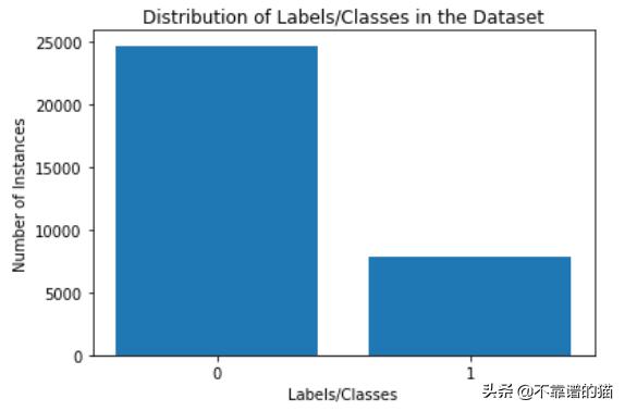
这里有两个类标签:0和1,是不平衡的
用这种不平衡的数据集训练机器学习模型,往往会导致模型对多数类产生一定的偏差,从而对少数类实例/数据点进行错误分类。
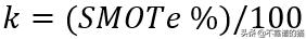
SMOTe是一种基于最近邻的技术,由欧几里德判断特征空间中的数据点之间的距离。过采样的百分比表示要创建的合成样本的数量,过采样的百分比参数始终是100的倍数。如果过采样的百分比是100,那么对于每个实例,新样本将被创建,因此,少数类实例的数量将增加一倍。同样,如果过采样的百分比是200,那么少数类样本的总数将增加到三倍。在SMOTe中,
- 对于每个少数类实例,找到k个最近邻,使得它们也属于同一个类,其中,
- 找到所考虑的实例的特征向量与k个最近邻的特征向量之间的差异。得到了k个不同向量。
- k个不同向量各自乘以0和1之间的随机数(不包括0和1)。
- 现在,向量在乘以随机数之后,在每次迭代时被添加到所考虑的实例(原始少数类实例)的特征向量中。
从头开始在Python中实现SMOTe如下 -
import numpy as npdef nearest_neighbour(X, x): euclidean = np.ones(X.shape[0]-1) additive = [None]*(1*X.shape[1]) additive = np.array(additive).reshape(1, X.shape[1]) k = 0 for j in range(0,X.shape[0]): if np.array_equal(X[j], x) == False: euclidean[k] = sqrt(sum((X[j]-x)**2)) k = k + 1 euclidean = np.sort(euclidean) weight = random.random() while(weight == 0): weight = random.random() additive = np.multiply(euclidean[:1],weight) return additive def SMOTE_100(X): new = [None]*(X.shape[0]*X.shape[1]) new = np.array(new).reshape(X.shape[0],X.shape[1]) k = 0 for i in range(0,X.shape[0]): additive = nearest_neighbour(X, X[i]) for j in range(0,1): new[k] = X[i] + additive[j] k = k + 1 return new # the synthetic samples created by SMOTe 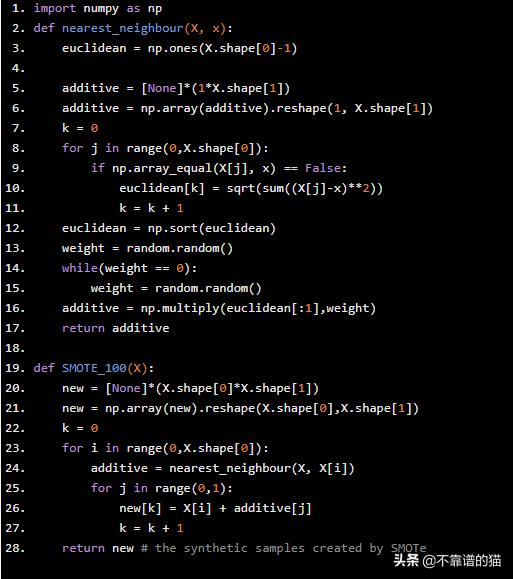
机器学习数据集
让我们考虑来自UCI(加州大学欧文分校)的Adult数据集(http://archive.ics.uci.edu/ml/datasets/Adult),其包含48,842个实例和14个属性/特征。
使用Python实现数据预处理:
- 标签编码是针对表1中提到的分类(非数字)特征和标签income进行的。
- 通过使用额外的树分类器对整个数据集进行训练进行特征选择,得到每个特征的特征重要性评分(由分类器给出),如表1所示。特征race和native-country 被删除,因为他们有最小的特征重要性得分。
- 对于具有两个以上类别的分类特征,执行One-Hot编码。在One-Hot编码之后,分类特征分成子特征,每个子特征对应于其类别之一,假设二进制值为0/1。在这里,分类特征,workclass, education, marital status, occupation 和 relationship是One-Hot编码。由于sex是一个只有2个子类别(男性和女性)的特征,因此不需要进一步编码。
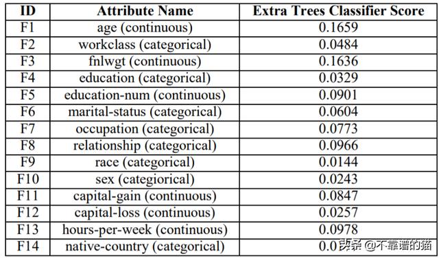
表格1
在特征选择后,在Python中实现One-Hot编码....
import numpy as npimport pandas as pdfrom sklearn.preprocessing import OneHotEncoder# Label Encoding and Feature Selection is over ....# 1. Loading the modified dataset after Label Encodingdf = pd.read_csv('adult.csv') # Loading of Selected Features into XX = df.iloc[:,[0,1,2,3,4,5,6,7,9,10,11,12]].values# Loading of the Label into yy = df.iloc[:,14].values# 2. One Hot Encoding ....onehotencoder = OneHotEncoder(categorical_features = [1,3,5,6,7])X = onehotencoder.fit_transform(X).toarray()
这个问题中的类标签是二进制的。这意味着类标签假设两个值,即有两个类。这是一个二元分类问题。
可视化类别分布
# Getting the no. of instances with Label 0n_class_0 = df[df['income']==0].shape[0]# Getting the no. of instances with label 1n_class_1 = df[df['income']==1].shape[0]# Bar Visualization of Class Distributionimport matplotlib.pyplot as plt # required libraryx = ['0', '1']y = np.array([n_class_0, n_class_1])plt.bar(x, y)plt.xlabel('Labels/Classes')plt.ylabel('Number of Instances')plt.title('Distribution of Labels/Classes in the Dataset')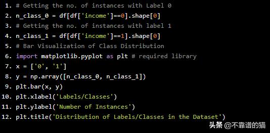
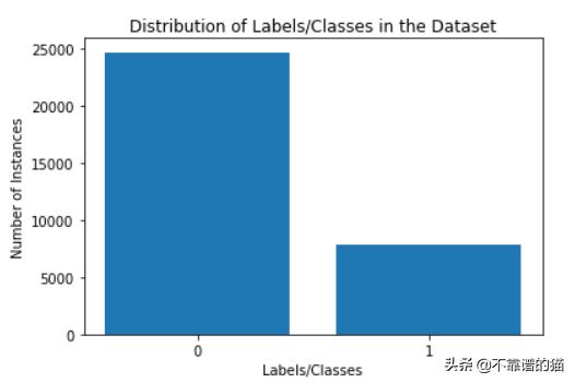
类分布
因此,在给定的数据集中,具有Class标签的两个类之间存在严重的不平衡,“1”为少数类,“0”为多数类。
现在,有两种可能的方法:
- 将数据集Shuffling并拆分为训练和验证集,并在训练数据集上应用SMOTe。(第1种方法)
- 将SMOTe作为整体应用于给定数据集,然后将机器学习数据集随机分割为训练和验证集。(第2种方法)
在Stack Overflow和许多个人博客等许多网络资源中,第二种方法被认为是过采样的错误方法。特别是,Nick Becker的个人博客中他提到第二种方法是错误的,原因如下:
“ SMOTe在整个数据集上的应用创建了类似的实例,因为该算法基于k-最近邻理论。由于这个原因,在对给定数据集应用SMOTe后进行拆分会导致信息从验证集泄漏到训练集,从而导致分类器或机器学习模型高估其准确性和其他性能指标 “
我们也用下第二种方法并进行一下比较。
让我们遵循第一种方法,因为它在整个过程中被广泛接受。
为了证明第二种方法没有错,我将把整个数据集随机分成训练验证和测试集。测试集将作为未知的实例集保持独立。
from sklearn.model_selection import train_test_split X_train, X_test, y_train, y_test = train_test_split(X, y, test_size=0.2, random_state=1234)# X_train and y_train is the Train-Validation Set# X_test and y_test is the Test Set separated out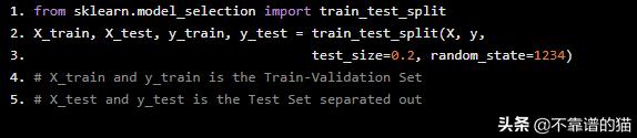
- 现在,在训练验证集中,第一和第二种方法将将应用case-wise。
- 对于这两种模型(按照第一种方法和第二种方法开发),将在同一分离的未知实例集(测试集)上进行性能分析
在拆分之后使用SMOTe的第一种方法
=>将训练验证集拆分为训练和验证集。Python代码如下:
X_train, X_v, y_train, y_v = train_test_split(X_train, y_train, test_size=0.2, random_state=2341)# X_train and y_train is the Training Set# X_v and y_v is the Validation Set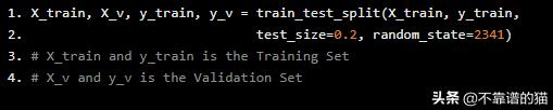
=>仅在训练集上应用SMOTe
# 1. Getting the number of Minority Class Instances in Training Setimport numpy as np # required libraryunique, counts = np.unique(y_train, return_counts=True)minority_shape = dict(zip(unique, counts))[1]# 2. Storing the minority class instances separatelyx1 = np.ones((minority_shape, X_train.shape[1]))k=0for i in range(0,X_train.shape[0]): if y_train[i] == 1.0: x1[k] = X[i] k = k + 1# 3. Applying 100% SMOTesampled_instances = SMOTE_100(x1)# Keeping the artificial instances and original instances togetherX_f = np.concatenate((X_train,sampled_instances), axis = 0)y_sampled_instances = np.ones(minority_shape)y_f = np.concatenate((y_train,y_sampled_instances), axis=0)# X_f and y_f are the Training Set Features and Labels respectively 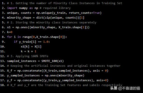
使用Gradient Boosting分类器进行模型训练
利用Gradient Boosting分类器对机器学习模型进行训练。Gradient Boosting分类器采用网格搜索的方法,得到了估计量和最大深度的最佳超参数集。
from sklearn.ensemble import GradientBoostingClassifierfrom sklearn.model_selection import GridSearchCVparameters = {'n_estimators':[100,150,200,250,300,350,400,450,500], 'max_depth':[3,4,5]}clf= GradientBoostingClassifier()grid_search = GridSearchCV(param_grid = parameters, estimator = clf, verbose = 3)grid_search_1 = grid_search.fit(X_f,y_f)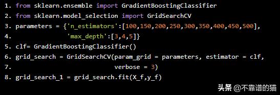
因此,第一种方法的训练机器学习模型嵌入在grid_search_1中。
以下是在拆分之前使用SMOTe的第二种方法
=>在整个训练验证集上应用SMOTe :
# 1. Getting the number of Minority Class Instances in Training Setunique, counts = np.unique(y_train, return_counts=True)minority_shape = dict(zip(unique, counts))[1]# 2. Storing the minority class instances separatelyx1 = np.ones((minority_shape, X_train.shape[1]))k=0for i in range(0,X_train.shape[0]): if y_train[i] == 1.0: x1[k] = X[i] k = k + 1# 3. Applying 100% SMOTesampled_instances = SMOTE_100(x1)# Keeping the artificial instances and original instances togetherX_f = np.concatenate((X_train,sampled_instances), axis = 0)y_sampled_instances = np.ones(minority_shape)y_f = np.concatenate((y_train,y_sampled_instances), axis=0)# X_f and y_f are the Train-Validation Set Features and Labels respectively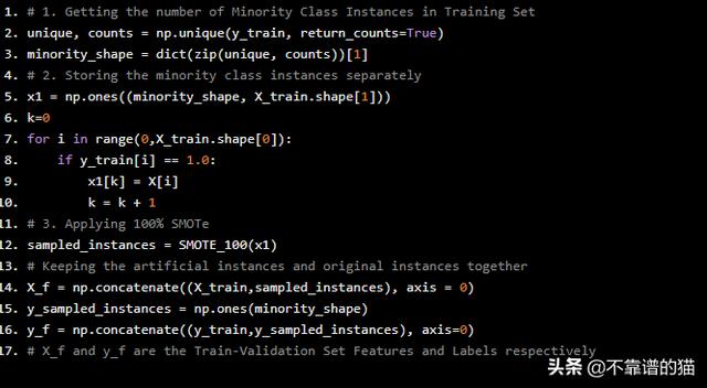
=>将训练验证集拆分为训练和验证集。
X_train, X_v, y_train, y_v = train_test_split(X_f, y_f, test_size=0.2, random_state=9999)# X_train and y_train is the Training Set# X_v and y_v is the Validation Set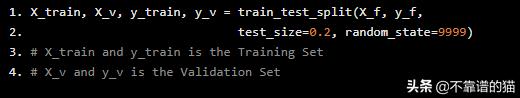
使用Gradient Boosting分类器进行模型训练
同样,Grid-Search也适用于Gradient Boosting Classifier
from sklearn.ensemble import GradientBoostingClassifierfrom sklearn.model_selection import GridSearchCVparameters = {'n_estimators':[100,150,200,250,300,350,400,450,500], 'max_depth':[3,4,5]}clf= GradientBoostingClassifier()grid_search = GridSearchCV(param_grid = parameters, estimator = clf, verbose = 3)grid_search_2 = grid_search.fit(X_train,y_train)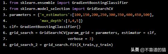
因此,第二种方法的训练机器学习模型嵌入在grid_search_2中。
分析与比较
用于比较和分析的绩效指标是:
- 测试集上的准确度
- 测试集上的精度
- 测试集上的Recall
- 测试集上的 F1-分数
除了这些比较指标之外,还计算训练准确度(训练集)和验证准确度(验证集)。
# MODEL 1 PERFORMANCE ANALYSIS# 1. Training Accuracy for Model 1 (following Approach 1)print(grid_search_1.score(X_f, y_f))# 2. Validation Accuracy on Validation Set for Model 1 print(grid_search_1.score(X_v, y_v))# 3. Test Accuracy on Test Set for Model 1print(grid_search_1.score(X_test, y_test))# 4. Precision, Recall and F1-Score on the Test Set for Model 1from sklearn.metrics import classification_reportpredictions=grid_search_1.predict(X_test)print(classification_report(y_test,predictions))# MODEL 2 PERFORMANCE ANALYSIS# 5. Training Accuracy for Model 2(following Approach 2)print(grid_search_2.score(X_train, y_train))# 6. Validation Accuracy on Validation Set for Model 2print(grid_search_2.score(X_v, y_v))# 3. Test Accuracy on Test Set for Model 2print(grid_search_2.score(X_test, y_test))# 4. Precision, Recall and F1-Score on the Test Set for Model 2from sklearn.metrics import classification_reportpredictions=grid_search_2.predict(X_test)print(classification_report(y_test,predictions))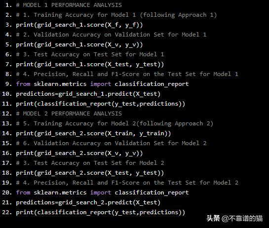
模型1和模型2的训练和验证集准确度为:
- 训练准确度(模型1):90.64998262078554%
- 训练准确度(模型2):90.92736479956705%
- 验证准确度(模型1):86.87140115163148%
- 验证准确度(模型2):89.33209647495362%
因此,从这里可以看出,第二种方法的验证准确率较高,但如果不对完全未知且相同的测试集进行测试,则无法得出结论。表2为两种模型在测试集上的性能对比图。
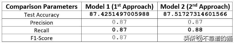
表2
所很明显,无论差异有多小,方法2显然比方法1更成功,这是什么原因?大家可以做下测试。
虽然SMOTe创建了类似的实例,但另一方面,这个属性不仅是为了减少类不平衡和数据增强,而且是为了找到最适合模型训练的训练集。
(二) kaggle 欺诈信用卡预测——不平衡训练样本的处理方法 综合结论就是:随机森林+过采样(直接复制或者smote后,黑白比例1:3 or 1:1)效果比较好!记得在smote前一定要先做标准化!!!


 3408
3408

 被折叠的 条评论
为什么被折叠?
被折叠的 条评论
为什么被折叠?
 到【灌水乐园】发言


