


| 时间 | 版本 | 修改人 | 描述 |
|---|---|---|---|
| 2023年11月15日11:17:27 | V0.1 | 宋全恒 | 新建文档 |
简介
softmax分享可以参考什么是softmax
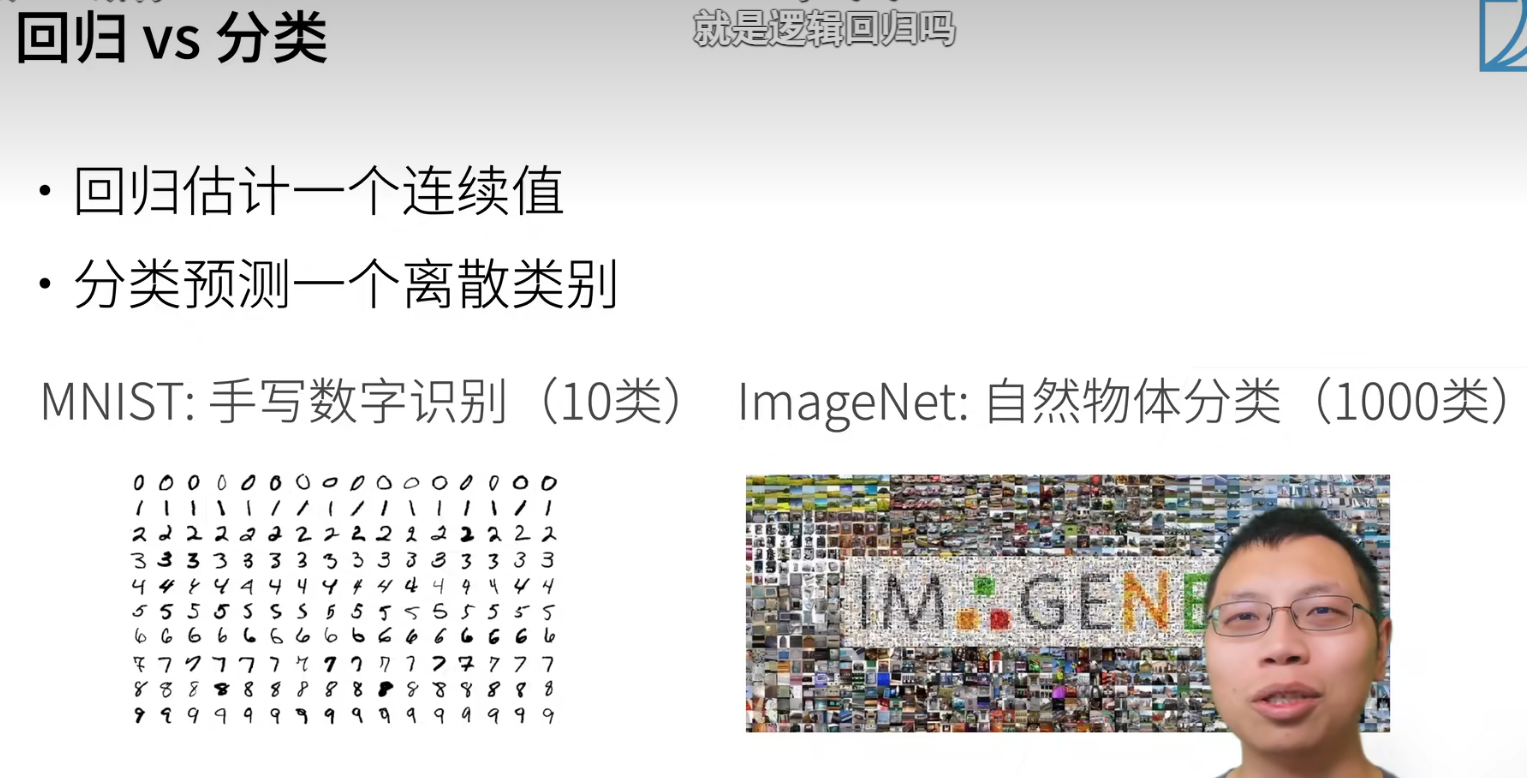
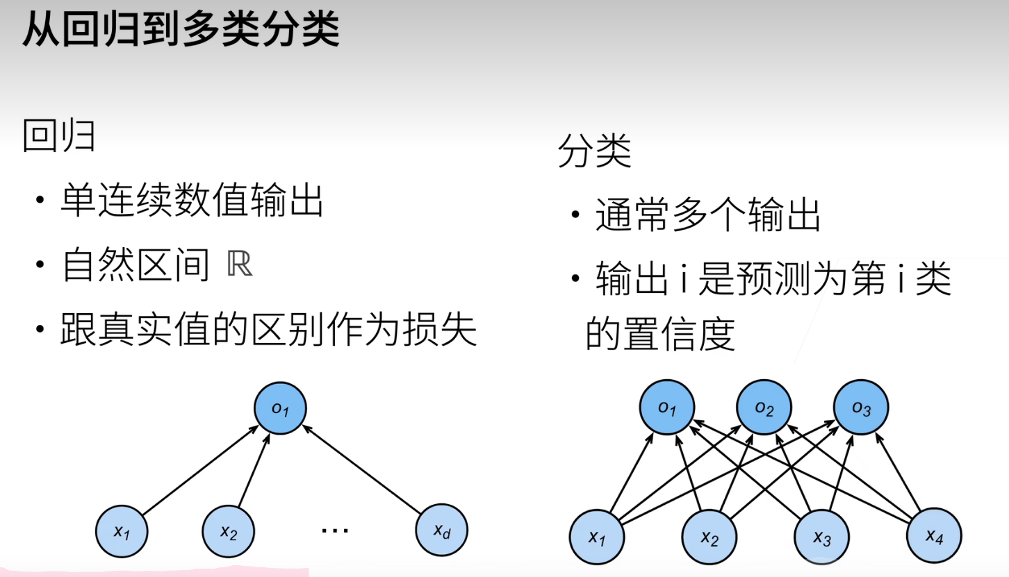
回归估计一个连续值,分类预测一个离散类别。
恶意软件的判断

回归和分类
分类可以认为从回归的单输出变成多输出
B站学习
softmax回归
使用softmax回归,解决多分类问题,softmax回归模型。
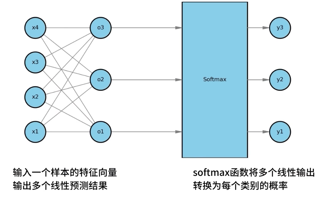

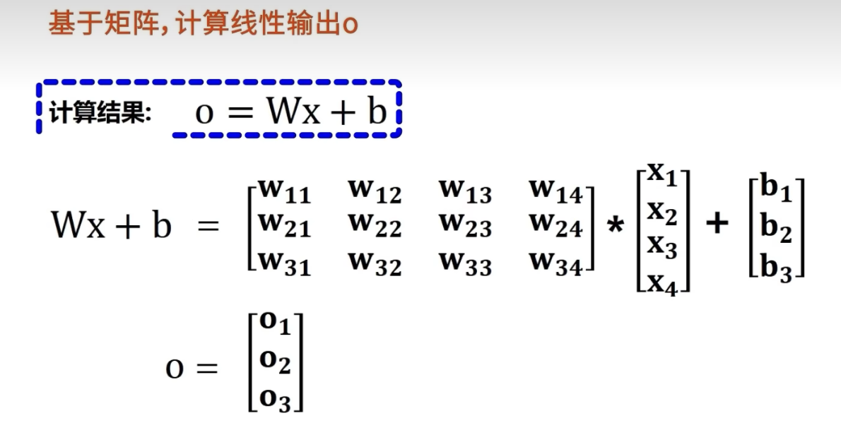
使用矩阵计算线性输出O
通过softmax计算概率:
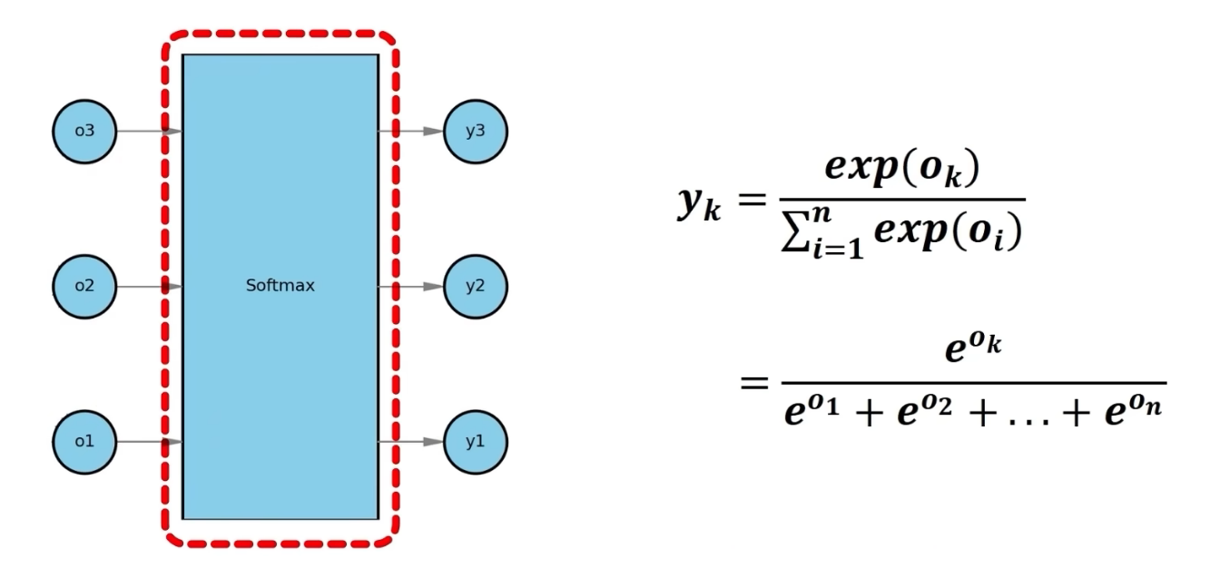
y值较大的概率属于相应类别的概率更高。
具体的计算过程如下图:

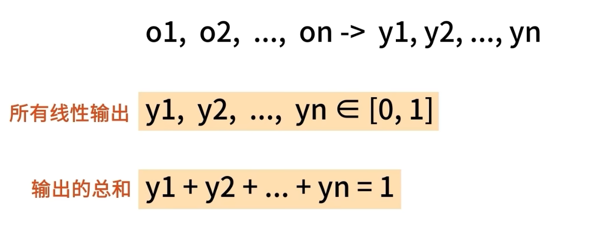
总结来说,softmax函数不会改变线性输出o之间的大小顺序,只会为每个类别分配相应的概率。softmax回归模型简介高效,只需要一次就能输出所有类别概率。

增加新的类别,产生较高的成本,以你为会影响所有的类别的概率。
softmax 回归+ 损失函数 + 图片分类数据集
均方损失训练。
Softmax
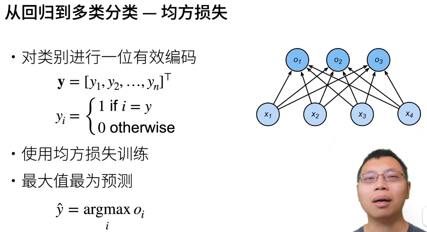
y ^ = a r g m a x o i \widehat { y } = a r g m a x o _ { i } y =argmaxoi
关注的不是o的输出,而是关注相对距离。
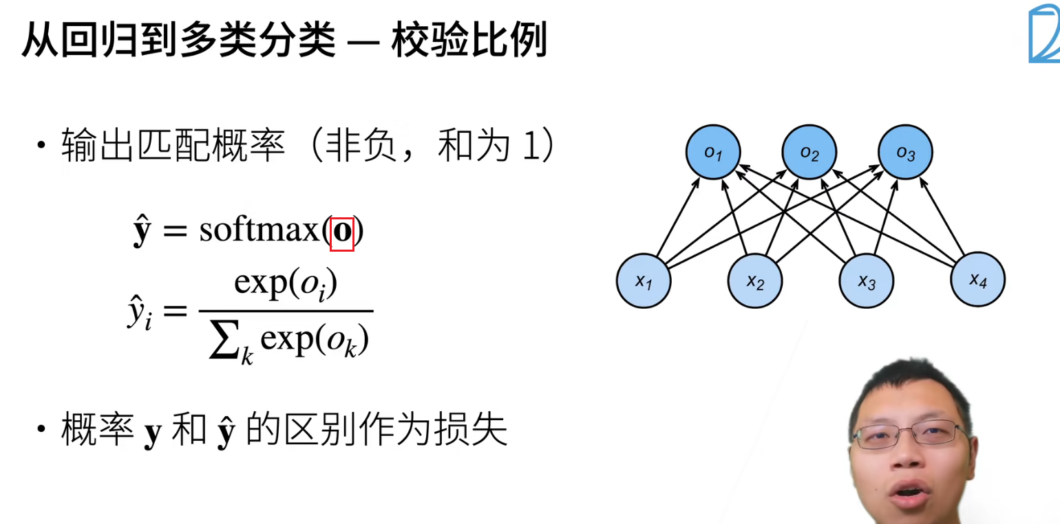
指数的好处,是具有非负性。
一般衡量两个概率的区别,使用交叉熵
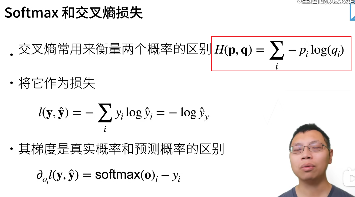
对真实类别的预测值,求其-log。
注: 上图是非常关键的,在计算交叉熵的时候,由于对应每个样本只有一个真实类别值为1,其他均为0,这样求和就可以表示为只有预测值的取log后,再取负数即可。
总结:
-
softmax回归是一个多类分类模型。
-
使用Softmax操作子得到每个类的预测置信度
-
使用交叉熵来衡量预测和标号的区别。
损失函数
损失函数是预测值和真实值的区别。
均方损失
1/2是为了求导时处理掉倍数。
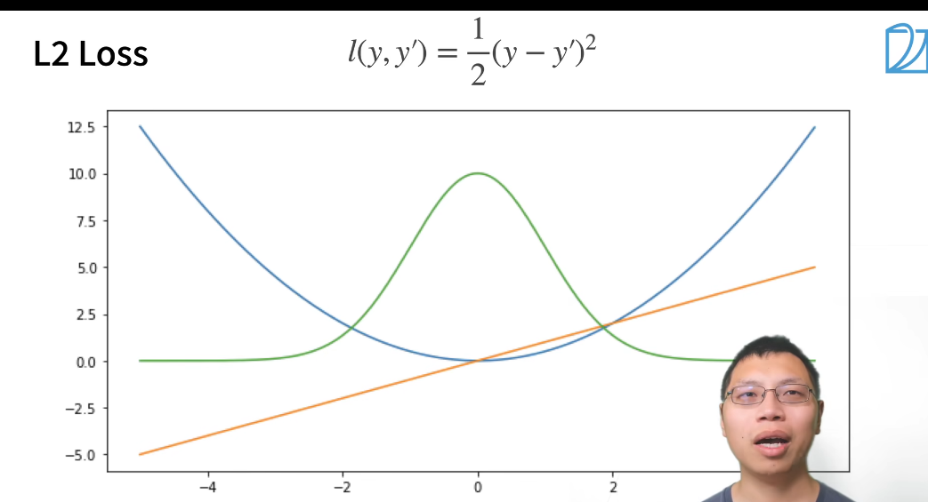
在负梯度方向更新参数。
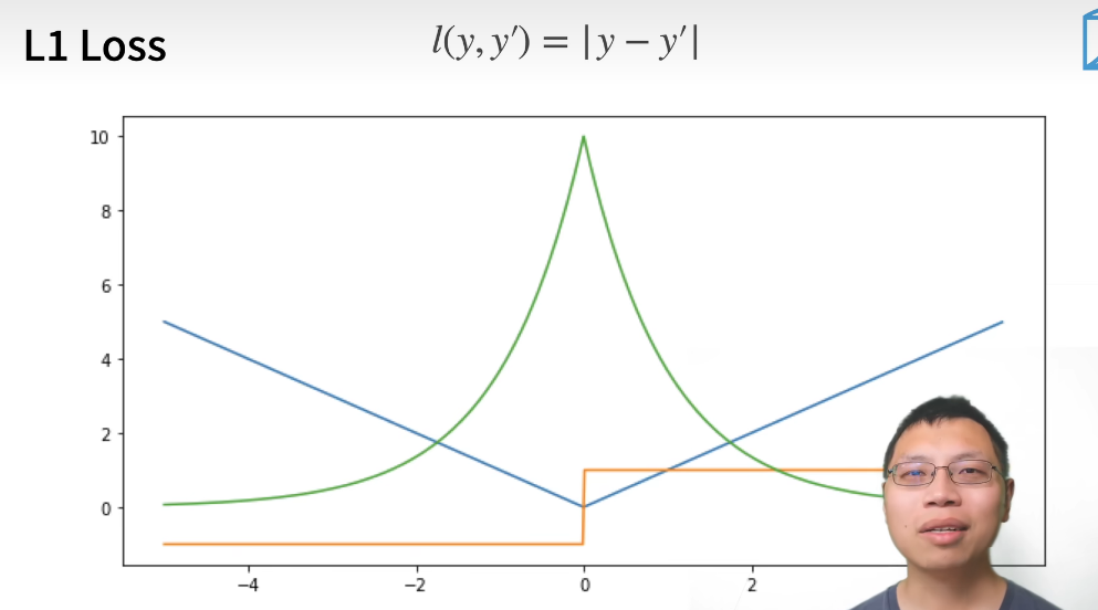
L1 loss
绿色的线是似然函数。
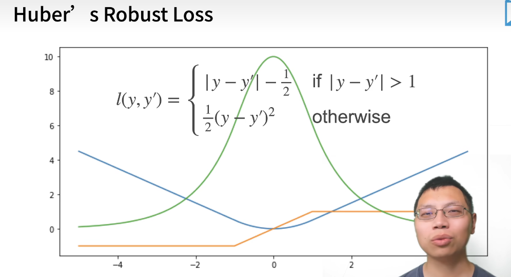
Hubers Robust Loss
当我预测值和真实值比较远时候,梯度是比较均匀的力度在靠近
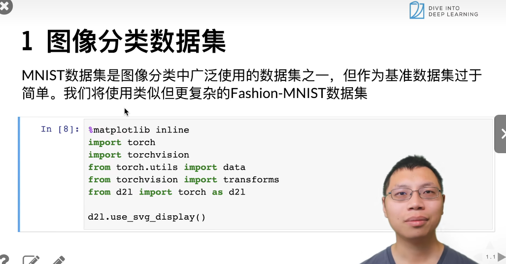
图像数据集
MNIST数据集是图像分类中广泛使用的数据集之一,但作为数据集过于简单。我们可以使用Fashin-MNIST作为数据集。
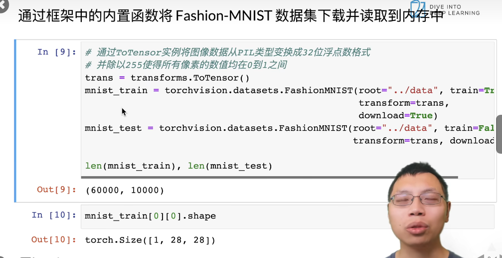
测试数据集用来验证模型的好坏
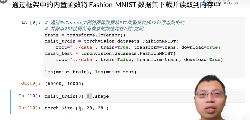
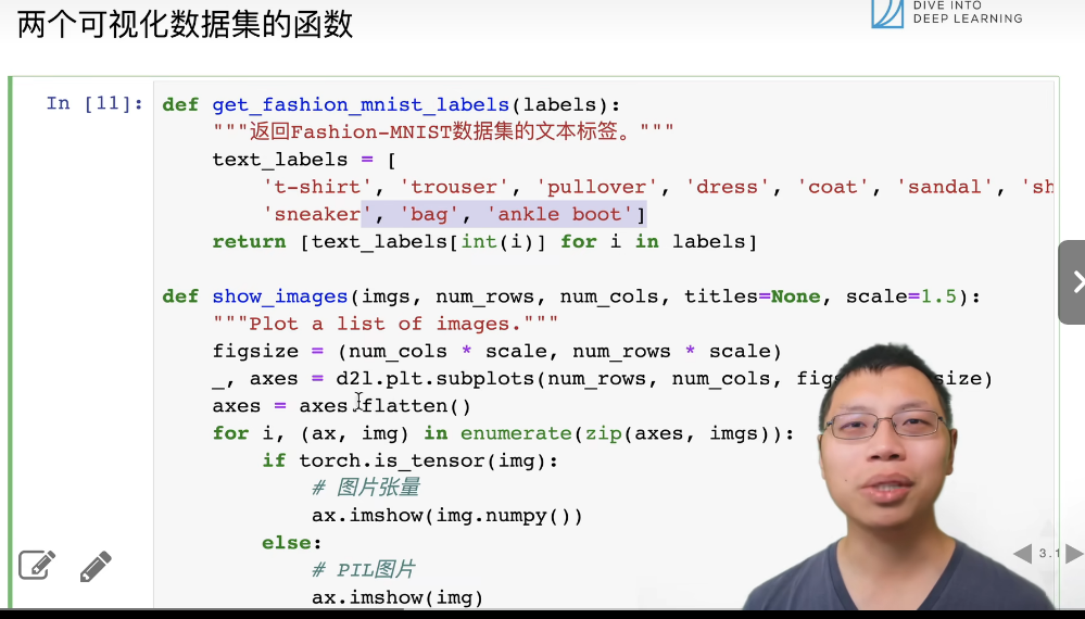
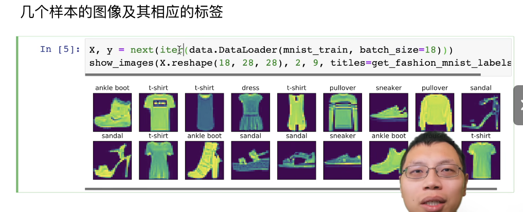
几个样本图像及相应的特征
读取进程数,来读取图像。shuffle,打乱顺序。
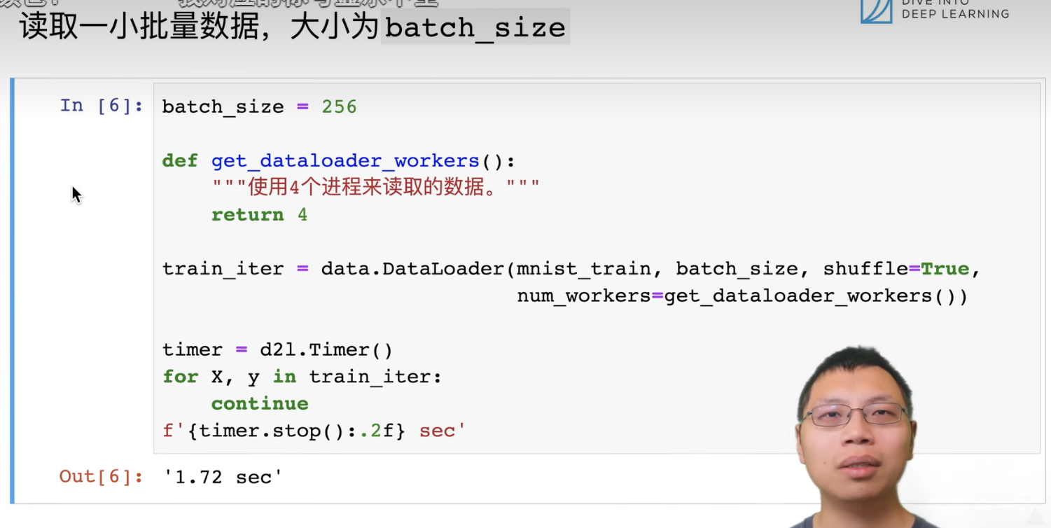
读一次数据要1.72秒。读取数据的速度。
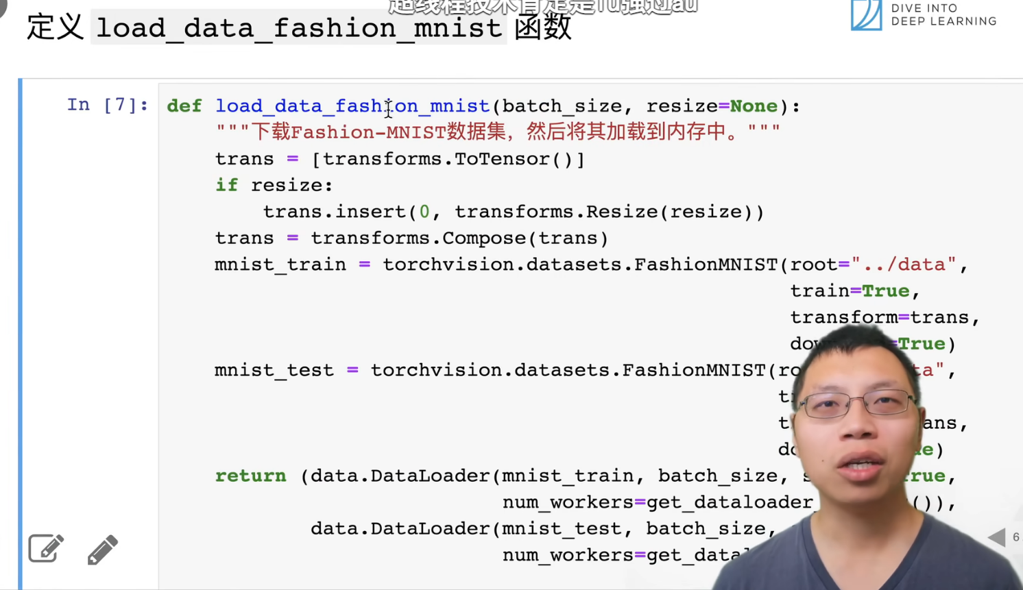
完整代码,定义load_data_fashion_mnist函数
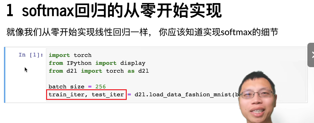
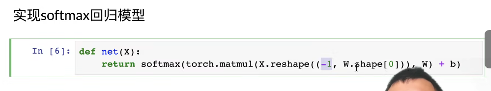
softmax回归从零开始实现
将展平每个图像,将它们视为784的向量,数据集一共10个类别,所以网络输出维度为10。
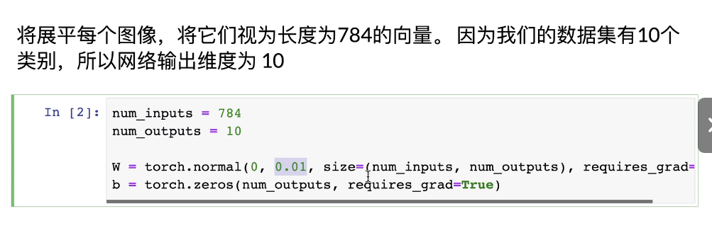
矩阵求和,维度等于0,将压缩成行详列。按照维度为1,将变成一个列向量。

实现softmax。
注: 对一个矩阵求softmax,相当于对其中的每一行求softmax,因为行数其实相当于样本数量了。也就是按照维度为1进行计算。
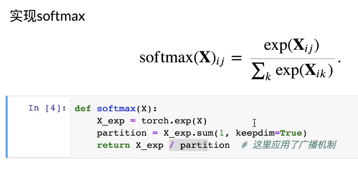
上述广播机制的含义是用矩阵的第i行,除以partition向量中的第i个值。
第一行是生成一个均值为0,方差为1的2行5列的矩阵。
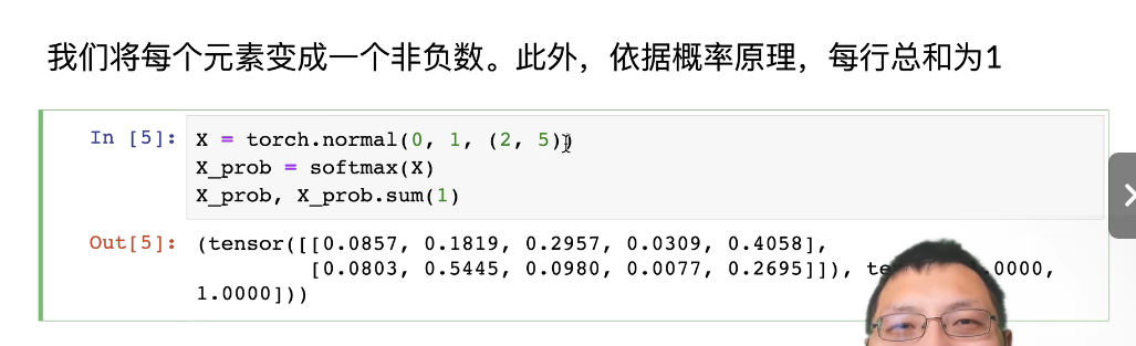
由结果,可以看出,每行的和为1,而且都是为正值。
计算交叉熵
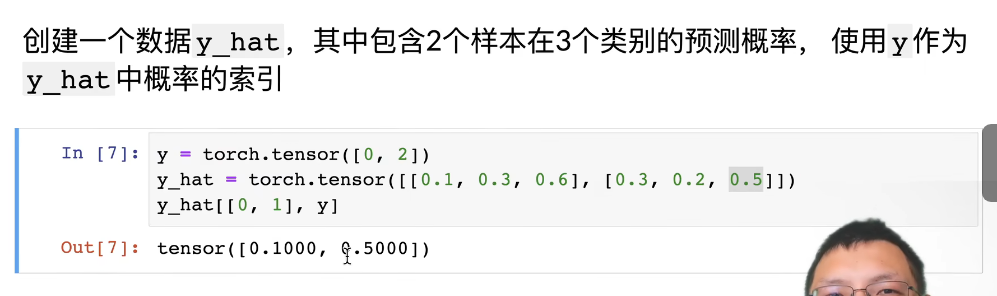
其中[0.1, 0.3, 0.6]是第一个样本的预测值。 y则表示两个样本的真实标签,第一个样本真实标签为0, 第二样本真实标签为2.
拿出0号样本和1号样本对应真实标签的预测值。y[1]为2,代表真实标签为2,然后取出预测为2的概率,即0.5。稍微有一点绕。在y_hat[[0,1], y]中[0, 1]代表了序号,即y向量中0号位和1号位的值,代表了真实的标签。y_hat则表示了对应这些类别的预测值。
实现交叉熵损失函数

计算预测准确的

找出预测正确的样本数。
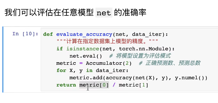
任意模型在数据迭代器的准确率
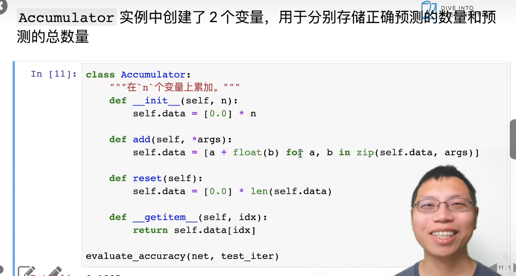
累加器
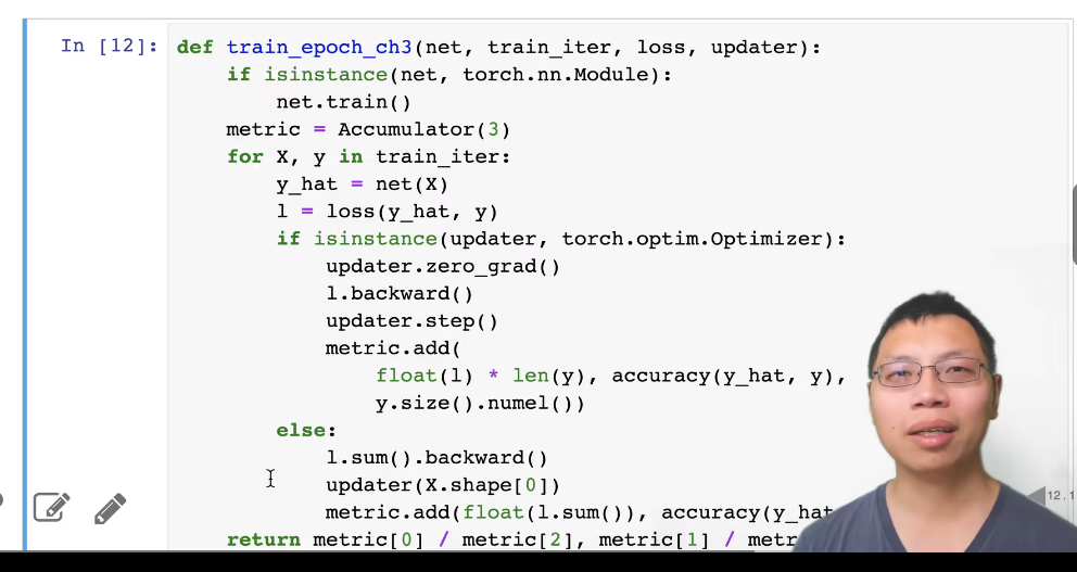
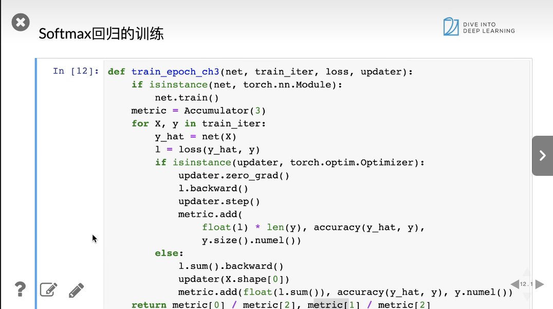
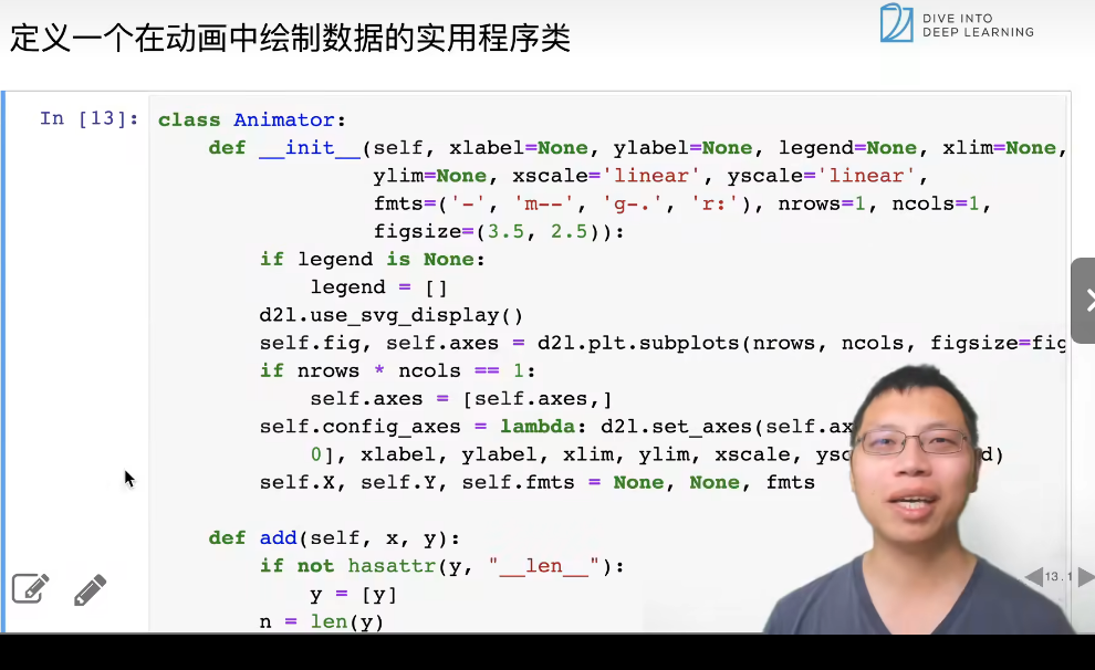
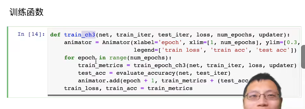
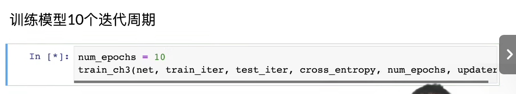
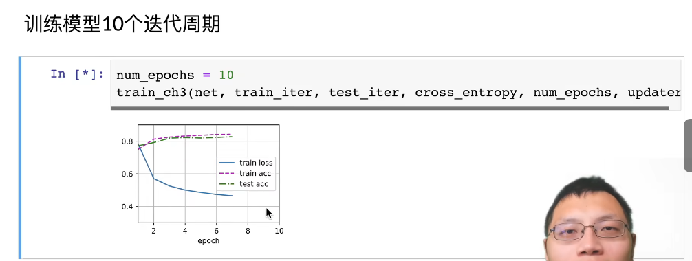
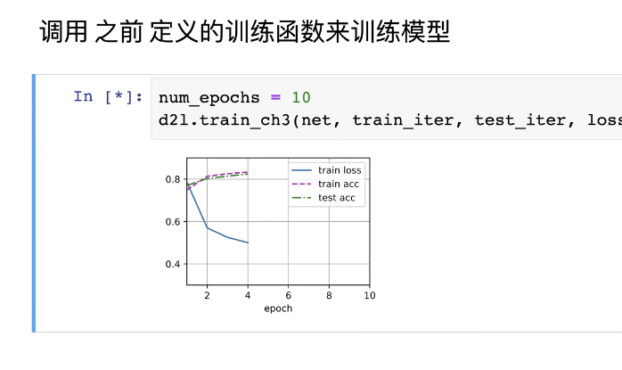
softmax回归的训练

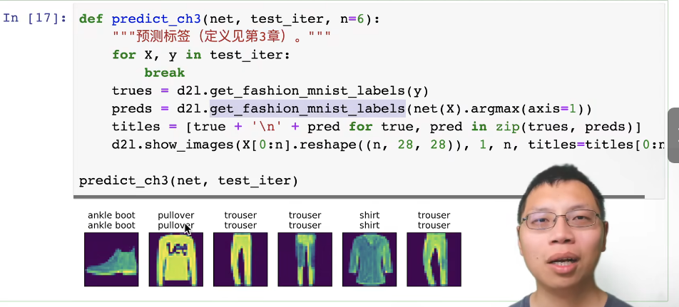
进行预测
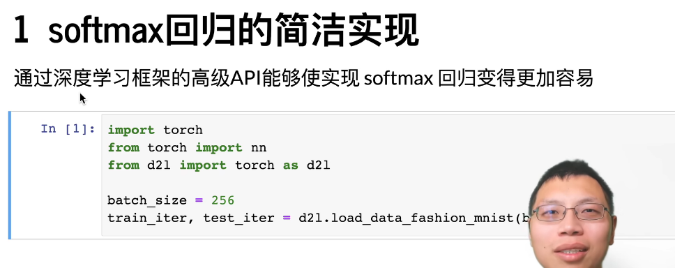
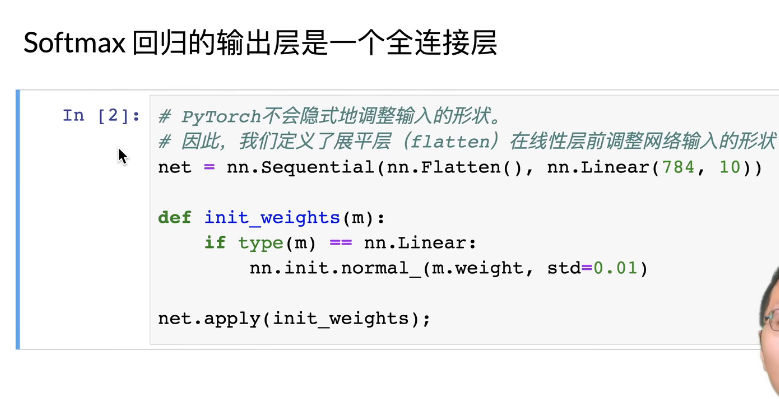
softmax简介实现

总结
softmax基本上是在多分类问题中,将输出概率化的操作子。在神经网络中,作为最后一层进行的。其中交叉熵的理解反而不太好。
cross_entropy = tf.nn.softmax_cross_entropy_with_logits(logits=layer_fc2, labels=y_true)
cost = tf.reduce_mean(cross_entropy)
optimizer = tf.train.AdamOptimizer(learning_rate=1e-4).minimize(cost)
correct_prediction = tf.equal(y_pred_cls, y_true_cls)
accuracy = tf.reduce_mean(tf.cast(correct_prediction, tf.float32))
session.run(tf.global_variables_initializer())
上述为在TF中使用交叉熵来获取准确率的样例代码,可以看到correct_prediction为一组向量[True, False, False, …]强制转化为tf.float32之后求平均,就相当于求出了准确率。
上图理解的关键是损失函数,其中y = [0, 0, …, 1, 0, 0]只有一个1,其他全为0,为1的索引为真实的类别标签。而y_hat = [0.1, 0.1, …, 0.3, 0.1, 0.1]都是一组预测的概率,这样在计算时,只要去取真实标签的预测值求-log即可得到该样本的损失。这相当于一个样本的误差。
不懂的东西太多了,之后买一本《动手学深度学习》好好看吧
最近有的时候很恐慌,因为在我的组里优秀的人很多,大家都在写论文什么的,自己呢深度学习比较浅显,就有点尴尬,其实一种治疗恐慌焦虑的方式就是深刻的意识到,知难则行易,知易则行难。所以别多想了,学就是了,另外如果担心做的贡献少的话,那就有多大能力做多少事情,做自己力所能及的所有事情,不要偷懒,认真学习就好了。2023年就要过去了,希望自己越来越好吧。希望每个读者都能够远离恐慌,规划好自己的人生,不要做错事,走错路,好好享受属于自己的人生。希望每段人生都是充实的,圆满的也。感恩一下。


 1097
1097


 被折叠的 条评论
为什么被折叠?
被折叠的 条评论
为什么被折叠?
 到【灌水乐园】发言


