阿里云天池龙珠计划深度学习训练营打卡-DCGAN生成微笑表情实战

 本笔记为阿里云天池龙珠计划深度学习训练营的学习内容,链接为:

AI训练营深度学习-阿里云天池

目录

1. 导入所需包

2. 基本参数配置

1. 导入数据集

2. 定义生成器与判别器

3. 初始化生成器和判别器

4. 定义损失函数

5. 开始训练

6. 绘制损失曲线

7. 真假对比

本项目使用 DCGAN 模型，在自建数据集上进行实验。

本项目使用的数据集是人脸嘴巴区域——微笑表情的数据集

​

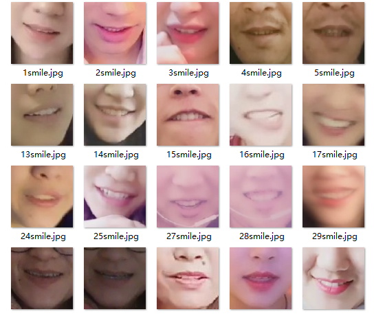
数据集文件夹结构如下，图片供 4357 张

├─mouth
│  └─smile
     ├─1smile.jpg
     ├─2smile.jpg
     ├─3smile.jpg
     └─....  

同时，创建一个 out 文件夹来保存训练的中间结果，主要就是看 DCGAN 是如何从一张噪声照片生成我们期待的图片

import os

import time

if os.path.exists("out"):

    print("移除现有 out 文件夹！")

    os.system("rm -r ./out")

time.sleep(1)

print("创建 out 文件夹！")

os.mkdir("./out")

移除现有 out 文件夹！

创建 out 文件夹！

1. 在加载该 NoteBook 文件时,会自动加载数据集至 ./download/mouth 文件夹下。若没有自动加载数据集，则需要手动加载，手动加载方式如下：

点击本页面左方 天池 按钮（需要在 CPU 环境下），点击 mouth 旁边的下载按钮，就会自动加载数据集了！ 

​

运行下面代码，对数据集进行解压。

由于图片数量多，解压需要一定时间

!unzip mouth.zip -d ./mouth

print("解压完毕！")

Archive:  mouth.zip

   creating: ./mouth/smile/

  inflating: ./mouth/smile/1000smile.jpg  

  inflating: ./mouth/smile/1001smile.jpg  

  inflating: ./mouth/smile/1002smile.jpg  

   ......  

导入所需包

from __future__ import print_function  # 在python2中使用python3的打印函数

import os  # 与操作系统进行交互

import random  # 创建随机数

import torch

import torch.nn as nn  # 导入torch的nn模块，用于构建神经网络的模型

import torch.nn.parallel  # 多个GPU时并行运行

import torch.optim as optim  # torch的各种优化器

import torch.utils.data  # data模块下的DataLoader类用于批量加载数据

import torchvision.datasets as dset  # 从文件夹读取数据集，或者从网络下载数据集

import torchvision.transforms as transforms  # 图像数据转换

import torchvision.utils as vutils  # 图像处理相关的工具函数

import numpy as np  # 用于数据的科学计算

import matplotlib.pyplot as plt  # 画图

import matplotlib.animation as animation  # 图片合成动画

from IPython.display import HTML  # HTML的方式展示动画

os.environ['KMP_DUPLICATE_LIB_OK'] = 'True'  # 通过os.environ设置环境变量'KMP_DUPLICATE_LIB_OK'为True，允许同时有多个OpenMP链接到程序

基本参数配置

# 设置一个随机种子，方便进行可重复性实验

manualSeed = 999

print("Random Seed: ", manualSeed)

random.seed(manualSeed)   # 设置python的随机数种子

torch.manual_seed(manualSeed)  # 设置torch的随机数种子

# 数据集所在路径

dataroot = "mouth/"

# 数据加载的进程数，0表示只有主进程加载数据，大于0表示指定数量的worker进程加载数据，主进程则不参与加载数据

workers = 0

# Batch size 大小

batch_size = 64

# Spatial size of training images. All images will be resized to this

# size using a transformer.

# 图片大小

image_size = 64

# 图片的通道数

nc = 3

# Size of z latent vector (i.e. size of generator input)

nz = 100

# Size of feature maps in generator

ngf = 64

# Size of feature maps in discriminator

ndf = 64

# Number of training epochs

num_epochs = 10

# Learning rate for optimizers

lr = 0.0003

# Beta1 hyperparam for Adam optimizers

beta1 = 0.5

# Number of GPUs available. Use 0 for CPU mode.

ngpu = 1

# Decide which device we want to run on

device = torch.device("cuda:0" if (torch.cuda.is_available() and ngpu > 0) else "cpu")

Random Seed:  999

导入数据集

# We can use an image folder dataset the way we have it setup.

# Create the dataset

dataset = dset.ImageFolder(root=dataroot,

                           transform=transforms.Compose([

                               transforms.Resize(image_size),

                               transforms.CenterCrop(image_size),

                               transforms.ToTensor(),  # 图像数据的取值范围[0,1]

                               transforms.Normalize((0.5, 0.5, 0.5), (0.5, 0.5, 0.5)),  # 归一化图像数据的取值范围[-1,1]

                           ]))

# Create the dataloader

dataloader = torch.utils.data.DataLoader(dataset, batch_size=batch_size,

                                         shuffle=True, num_workers=workers)

简单看一下我们的原始数据集长啥样

# Plot some training images

real_batch = next(iter(dataloader))

plt.figure(figsize=(8,8))

plt.axis("off")

plt.title("Training Images")

# normalize=True将图像归一化到(0,1)，通过减去最小像素值并除以最大像素值
# to(device)将数据复制到GPU下处理性能更高，之后再通过cpu()将数据复制到CPU下以执行numpy命令
plt.imshow(np.transpose(vutils.make_grid(real_batch[0].to(device)[:64], padding=2, normalize=True).cpu(),(1,2,0)))

# plt.show()

[5]:

<matplotlib.image.AxesImage at 0x7f67b59d9cf8>

​

定义生成器与判别器

# 权重初始化函数，为生成器和判别器模型初始化

def weights_init(m):

    classname = m.__class__.__name__  # 取得模块的名称

    if classname.find('Conv') != -1:

        nn.init.normal_(m.weight.data, 0.0, 0.02)  # 卷积层的权重初始化为均值0，标准差0.02的正态随机数

    elif classname.find('BatchNorm') != -1:

        nn.init.normal_(m.weight.data, 1.0, 0.02)  # 归一化层的权重初始化为均值1，标准差0.02的正态随机数

        nn.init.constant_(m.bias.data, 0)  # 归一化层的偏置初始化为0

# Generator Code

class Generator(nn.Module):

    def __init__(self, ngpu):

        super(Generator, self).__init__()

        self.ngpu = ngpu

        self.main = nn.Sequential(

            # input is Z, going into a convolution

                          # 因为归一化层中添加偏置，所以卷积层不加偏置

            nn.ConvTranspose2d( nz, ngf * 8, 4, 1, 0, bias=False),  

            nn.BatchNorm2d(ngf * 8),

            nn.ReLU(True),  # 激活输出覆盖原有数据

            # state size. (ngf*8) x 4 x 4

            nn.ConvTranspose2d(ngf * 8, ngf * 4, 4, 2, 1, bias=False),

            nn.BatchNorm2d(ngf * 4),

            nn.ReLU(True),

            # state size. (ngf*4) x 8 x 8

            nn.ConvTranspose2d( ngf * 4, ngf * 2, 4, 2, 1, bias=False),

            nn.BatchNorm2d(ngf * 2),

            nn.ReLU(True),

            # state size. (ngf*2) x 16 x 16

            nn.ConvTranspose2d( ngf * 2, ngf, 4, 2, 1, bias=False),

            nn.BatchNorm2d(ngf),

            nn.ReLU(True),

            # state size. (ngf) x 32 x 32

            nn.ConvTranspose2d( ngf, nc, 4, 2, 1, bias=False),

            nn.Tanh()  # Tanh激活的输出值范围[-1,1]

            # state size. (nc) x 64 x 64

        )

    def forward(self, input):

        return self.main(input)

​

class Discriminator(nn.Module):

    def __init__(self, ngpu):

        super(Discriminator, self).__init__()

        self.ngpu = ngpu

        self.main = nn.Sequential(

            # input is (nc) x 64 x 64

            nn.Conv2d(nc, ndf, 4, 2, 1, bias=False),

            nn.LeakyReLU(0.2, inplace=True),  # 因为真实数据和生成器生成数据的值范围均是[-1,1]，所以这里用LeakyReLU激活

            # state size. (ndf) x 32 x 32

            nn.Conv2d(ndf, ndf * 2, 4, 2, 1, bias=False),

            nn.BatchNorm2d(ndf * 2),

            nn.LeakyReLU(0.2, inplace=True),

            # state size. (ndf*2) x 16 x 16

            nn.Conv2d(ndf * 2, ndf * 4, 4, 2, 1, bias=False),

            nn.BatchNorm2d(ndf * 4),

            nn.LeakyReLU(0.2, inplace=True),

            # state size. (ndf*4) x 8 x 8

            nn.Conv2d(ndf * 4, ndf * 8, 4, 2, 1, bias=False),

            nn.BatchNorm2d(ndf * 8),

            nn.LeakyReLU(0.2, inplace=True),

            # state size. (ndf*8) x 4 x 4

            nn.Conv2d(ndf * 8, 1, 4, 1, 0, bias=False),

            nn.Sigmoid()  # Sigmoid激活的输出值范围[0,1]

        )

    def forward(self, input):

        return self.main(input)

​

初始化生成器和判别器

# Create the generator

netG = Generator(ngpu).to(device)

# Handle multi-gpu if desired

if (device.type == 'cuda') and (ngpu > 1):

    netG = nn.DataParallel(netG, list(range(ngpu)))

# Apply the weights_init function to randomly initialize all weights

# to mean=0, stdev=0.2.

netG.apply(weights_init)  # apply函数先递归应用于netG的各子模块，再应用于netG模块自身

# Print the model

print(netG)

# Create the Discriminator

netD = Discriminator(ngpu).to(device)

# Handle multi-gpu if desired

if (device.type == 'cuda') and (ngpu > 1):

    netD = nn.DataParallel(netD, list(range(ngpu)))

# Apply the weights_init function to randomly initialize all weights

#  to mean=0, stdev=0.2.

netD.apply(weights_init)

# Print the model

print(netD)

Generator(

  (main): Sequential(

    (0): ConvTranspose2d(100, 512, kernel_size=(4, 4), stride=(1, 1), bias=False)

    (1): BatchNorm2d(512, eps=1e-05, momentum=0.1, affine=True, track_running_stats=True)

    (2): ReLU(inplace=True)

    (3): ConvTranspose2d(512, 256, kernel_size=(4, 4), stride=(2, 2), padding=(1, 1), bias=False)

    (4): BatchNorm2d(256, eps=1e-05, momentum=0.1, affine=True, track_running_stats=True)

    (5): ReLU(inplace=True)

    (6): ConvTranspose2d(256, 128, kernel_size=(4, 4), stride=(2, 2), padding=(1, 1), bias=False)

    (7): BatchNorm2d(128, eps=1e-05, momentum=0.1, affine=True, track_running_stats=True)

    (8): ReLU(inplace=True)

    (9): ConvTranspose2d(128, 64, kernel_size=(4, 4), stride=(2, 2), padding=(1, 1), bias=False)

    (10): BatchNorm2d(64, eps=1e-05, momentum=0.1, affine=True, track_running_stats=True)

    (11): ReLU(inplace=True)

    (12): ConvTranspose2d(64, 3, kernel_size=(4, 4), stride=(2, 2), padding=(1, 1), bias=False)

    (13): Tanh()

  )

)

Discriminator(

  (main): Sequential(

    (0): Conv2d(3, 64, kernel_size=(4, 4), stride=(2, 2), padding=(1, 1), bias=False)

    (1): LeakyReLU(negative_slope=0.2, inplace=True)

    (2): Conv2d(64, 128, kernel_size=(4, 4), stride=(2, 2), padding=(1, 1), bias=False)

    (3): BatchNorm2d(128, eps=1e-05, momentum=0.1, affine=True, track_running_stats=True)

    (4): LeakyReLU(negative_slope=0.2, inplace=True)

    (5): Conv2d(128, 256, kernel_size=(4, 4), stride=(2, 2), padding=(1, 1), bias=False)

    (6): BatchNorm2d(256, eps=1e-05, momentum=0.1, affine=True, track_running_stats=True)

    (7): LeakyReLU(negative_slope=0.2, inplace=True)

    (8): Conv2d(256, 512, kernel_size=(4, 4), stride=(2, 2), padding=(1, 1), bias=False)

    (9): BatchNorm2d(512, eps=1e-05, momentum=0.1, affine=True, track_running_stats=True)

    (10): LeakyReLU(negative_slope=0.2, inplace=True)

    (11): Conv2d(512, 1, kernel_size=(4, 4), stride=(1, 1), bias=False)

    (12): Sigmoid()

  )

)

定义损失函数

# Initialize BCELoss function

criterion = nn.BCELoss()

开始训练

# Create batch of latent vectors that we will use to visualize

#  the progression of the generator

fixed_noise = torch.randn(64, nz, 1, 1, device=device)

# Establish convention for real and fake labels during training

real_label = 1.0

fake_label = 0.0

# Setup Adam optimizers for both G and D

optimizerD = optim.Adam(netD.parameters(), lr=lr, betas=(beta1, 0.999))

optimizerG = optim.Adam(netG.parameters(), lr=lr, betas=(beta1, 0.999))

# Training Loop

# Lists to keep track of progress

img_list = []  # 存储生成器在噪声上生成的图像

G_losses = []

D_losses = []

iters = 0  # 存储迭代的总次数

print("Starting Training Loop...")

# For each epoch

for epoch in range(num_epochs):

    import time

    start = time.time()

    # For each batch in the dataloader

    for i, data in enumerate(dataloader, 0):  # 为批量加载的数据生成枚举值，从0开始

        ############################

        # (1) Update D network: maximize log(D(x)) + log(1 - D(G(z)))

        ###########################

        ## Train with all-real batch

        netD.zero_grad()  # 每批数据训练前，清除判别器参数的梯度

        # Format batch

        real_cpu = data[0].to(device)

        b_size = real_cpu.size(0)

        label = torch.full((b_size,), real_label, device=device)

        # Forward pass real batch through D

        output = netD(real_cpu).view(-1)  # 将批量真实数据输入判别器，并将输出展开为1维数据，用于和label计算损失

        # Calculate loss on all-real batch

        errD_real = criterion(output, label)

        # Calculate gradients for D in backward pass

        errD_real.backward()  # 反向传播计算判别器参数的梯度，此时也会计算生成器参数的梯度

        D_x = output.mean().item()  # 计算判别器基于批量真实数据的输出均值

        ## Train with all-fake batch

        # Generate batch of latent vectors

        noise = torch.randn(b_size, nz, 1, 1, device=device)

        # Generate fake image batch with G

        fake = netG(noise)

        label.fill_(fake_label)

        # Classify all fake batch with D

        output = netD(fake.detach()).view(-1)  # 不计算生成器参数的梯度

        # Calculate D's loss on the all-fake batch

        errD_fake = criterion(output, label)

        # Calculate the gradients for this batch

        errD_fake.backward()  # 累计判别器基于批量假数据的梯度

        D_G_z1 = output.mean().item()  # 判别器基于噪声生成假数据的输出

        # Add the gradients from the all-real and all-fake batches

        errD = errD_real + errD_fake

        # Update D

        optimizerD.step()  # 更新判别器的参数

        ############################

        # (2) Update G network: maximize log(D(G(z)))

        ###########################

        netG.zero_grad()  # 每批数据训练前，清除生成器参数的梯度

        label.fill_(real_label)  # fake labels are real for generator cost，此处是训练生成器，所有输入判别器的数据都是通过生成器生成的，因此输出标签为真

        # Since we just updated D, perform another forward pass of all-fake batch through D

        output = netD(fake).view(-1)

        # Calculate G's loss based on this output

        errG = criterion(output, label)

        # Calculate gradients for G

        errG.backward()  # 计算生成器参数的梯度

        D_G_z2 = output.mean().item()  # 计算判别器输出的均值，与D_G_z1之间相差一次参数更新

        # Update G

        optimizerG.step()  # 更新生成器参数

        # Output training stats

        if i % 50 == 0:  # 每训练50个批量

                          # 占位符：%d输出一个整数，%f输出一个浮点数

            print('[%d/%d][%d/%d]\tLoss_D: %.4f\tLoss_G: %.4f\tD(x): %.4f\tD(G(z)): %.4f / %.4f'

                  % (epoch, num_epochs, i, len(dataloader),

                     errD.item(), errG.item(), D_x, D_G_z1, D_G_z2))

        # Save Losses for plotting later

        G_losses.append(errG.item())  # 存储每个批量的生成器损失

        D_losses.append(errD.item())  # 存储每个批量的判别器损失

        # Check how the generator is doing by saving G's output on fixed_noise

        if (iters % 20 == 0) or ((epoch == num_epochs-1) and (i == len(dataloader)-1)):  # 如果迭代次数为20的整数倍，或者为最后一轮的最后一个批量

            with torch.no_grad():

                fake = netG(fixed_noise).detach().cpu()  # 得到生成器生成的假数据，无需生成计算图

                          # 将生成的假数据合成一个网格图像

            img_list.append(vutils.make_grid(fake, padding=2, normalize=True))

            i = vutils.make_grid(fake, padding=2, normalize=True)

            fig = plt.figure(figsize=(8, 8))

            plt.imshow(np.transpose(i, (1, 2, 0)))

            plt.axis('off')  # 关闭坐标轴

            plt.savefig("out/%d_%d.png" % (epoch, iters))  # 保存每个批量的图片

            plt.close(fig)

        iters += 1  # 每个批量训练结束后，将总迭代次数加1

    print('time:', time.time() - start)  # 打印每一轮训练消耗的时间

Starting Training Loop...

[0/10][0/69]	Loss_D: 1.6922	Loss_G: 10.4924	D(x): 0.6837	D(G(z)): 0.6499 / 0.0001

[0/10][50/69]	Loss_D: 0.0341	Loss_G: 35.9770	D(x): 0.9844	D(G(z)): 0.0000 / 0.0000

time: 45.65119695663452

[1/10][0/69]	Loss_D: 0.0003	Loss_G: 33.8338	D(x): 0.9997	D(G(z)): 0.0000 / 0.0000

[1/10][50/69]	Loss_D: 1.9597	Loss_G: 5.1042	D(x): 0.4813	D(G(z)): 0.0540 / 0.0197

time: 34.60388779640198

[2/10][0/69]	Loss_D: 1.7999	Loss_G: 4.8677	D(x): 0.5162	D(G(z)): 0.1226 / 0.0610

[2/10][50/69]	Loss_D: 1.0036	Loss_G: 6.6382	D(x): 0.4950	D(G(z)): 0.0013 / 0.0036

time: 34.82605242729187

[3/10][0/69]	Loss_D: 0.9899	Loss_G: 0.9510	D(x): 0.5255	D(G(z)): 0.0657 / 0.4808

[3/10][50/69]	Loss_D: 0.8487	Loss_G: 8.4878	D(x): 0.8906	D(G(z)): 0.4741 / 0.0006

time: 34.656062841415405

[4/10][0/69]	Loss_D: 0.6986	Loss_G: 10.3000	D(x): 0.9097	D(G(z)): 0.3872 / 0.0001

[4/10][50/69]	Loss_D: 0.4653	Loss_G: 4.1558	D(x): 0.7023	D(G(z)): 0.0290 / 0.0211

time: 34.64480686187744

[5/10][0/69]	Loss_D: 1.7700	Loss_G: 7.7769	D(x): 0.9840	D(G(z)): 0.7115 / 0.0040

[5/10][50/69]	Loss_D: 0.4862	Loss_G: 3.7039	D(x): 0.7550	D(G(z)): 0.0594 / 0.0549

time: 34.73557090759277

[6/10][0/69]	Loss_D: 1.1480	Loss_G: 7.8190	D(x): 0.8646	D(G(z)): 0.4626 / 0.0020

[6/10][50/69]	Loss_D: 1.6766	Loss_G: 5.0127	D(x): 0.3481	D(G(z)): 0.0024 / 0.0230

time: 36.48115563392639

[7/10][0/69]	Loss_D: 2.0191	Loss_G: 12.2408	D(x): 0.9676	D(G(z)): 0.7749 / 0.0000

[7/10][50/69]	Loss_D: 0.7136	Loss_G: 2.0795	D(x): 0.6281	D(G(z)): 0.1049 / 0.1796

time: 35.35510182380676

[8/10][0/69]	Loss_D: 2.1591	Loss_G: 2.8655	D(x): 0.2812	D(G(z)): 0.0124 / 0.1683

[8/10][50/69]	Loss_D: 1.7478	Loss_G: 2.6480	D(x): 0.3129	D(G(z)): 0.0105 / 0.1575

time: 36.06704092025757

[9/10][0/69]	Loss_D: 4.0272	Loss_G: 1.3274	D(x): 0.1171	D(G(z)): 0.0385 / 0.4230

[9/10][50/69]	Loss_D: 0.5768	Loss_G: 3.1357	D(x): 0.8594	D(G(z)): 0.2893 / 0.0799

time: 35.28251338005066

绘制损失曲线

plt.figure(figsize=(10,5))

plt.title("Generator and Discriminator Loss During Training")

plt.plot(G_losses,label="G")

plt.plot(D_losses,label="D")

plt.xlabel("iterations")

plt.ylabel("Loss")

plt.legend()

plt.show()

​

真假对比

# Grab a batch of real images from the dataloader

# real_batch = next(iter(dataloader))

# Plot the real images

plt.figure(figsize=(15,15))

plt.subplot(1,2,1)

plt.axis("off")

plt.title("Real Images")

plt.imshow(np.transpose(vutils.make_grid(real_batch[0].to(device)[:64], padding=5, normalize=True).cpu(),(1,2,0)))

# Plot the fake images from the last epoch

plt.subplot(1,2,2)

plt.axis("off")

plt.title("Fake Images")

plt.imshow(np.transpose(img_list[-1],(1,2,0)))

plt.show()

​