


本笔记为阿里云天池龙珠计划数据挖掘训练营的学习内容,链接为:
五、模型融合
Tip:此部分为零基础入门数据挖掘的 Task5 模型融合部分,带你来了解各种模型结果的融合方式,在比赛的攻坚时刻冲刺Top,欢迎大家后续多多交流。
赛题:零基础入门数据挖掘 - 二手车交易价格预测
地址:零基础入门数据挖掘 - 二手车交易价格预测_学习赛_天池大赛-阿里云天池的赛制
5.1 模型融合目标
-
对于多种调参完成的模型进行模型融合。
-
完成对于多种模型的融合,提交融合结果并打卡。
5.2 内容介绍
模型融合是比赛后期一个重要的环节,大体来说有如下的类型方式。
- 简单加权融合:
- 回归(分类概率):算术平均融合(Arithmetic mean),几何平均融合(Geometric mean);
- 分类:投票(Voting)
- 综合:排序融合(Rank averaging),log融合
- stacking/blending:
- 构建多层模型,并利用预测结果再拟合预测。
- boosting/bagging(在xgboost,Adaboost,GBDT中已经用到):
- 多树的提升方法
5.3 Stacking相关理论介绍
1) 什么是 stacking
简单来说 stacking 就是当用初始训练数据学习出若干个基学习器后,将这几个学习器的预测结果作为新的训练集,来学习一个新的学习器。
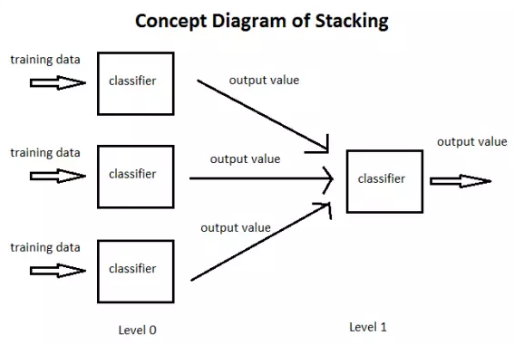
将个体学习器结合在一起的时候使用的方法叫做结合策略。对于分类问题,我们可以使用投票法来选择输出最多的类。对于回归问题,我们可以将分类器输出的结果求平均值。
上面说的投票法和平均法都是很有效的结合策略,还有一种结合策略是使用另外一个机器学习算法来将个体机器学习器的结果结合在一起,这个方法就是Stacking。(Stacking适用于分类和回归)
在stacking方法中,我们把个体学习器叫做初级学习器,用于结合的学习器叫做次级学习器或元学习器(meta-learner),次级学习器用于训练的数据叫做次级训练集。次级训练集是在训练集上用初级学习器得到的。
2) 如何进行 stacking
算法示意图如下:
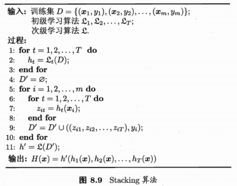
引用自 西瓜书《机器学习》
- 过程1-3 是训练出来个体学习器,也就是初级学习器。
- 过程5-9是 使用训练出来的个体学习器来获得预测的结果,这个预测的结果当做次级学习器的训练集。
- 过程11 是用初级学习器预测的结果训练出次级学习器,得到我们最后训练的模型。
3)Stacking的方法讲解
首先,我们先从一种“不那么正确”但是容易懂的Stacking方法讲起。
Stacking模型本质上是一种分层的结构,这里简单起见,只分析二级Stacking.假设我们有2个基模型 Model1_1、Model1_2 和 一个次级模型Model2
Step 1. 基模型 Model1_1,对训练集train训练,然后用于预测 train 和 test 的标签列,分别是P1,T1
Model1_1 模型训练:

训练后的模型 Model1_1 分别在 train 和 test 上预测,得到预测标签分别是P1,T1

Step 2. 基模型 Model1_2 ,对训练集train训练,然后用于预测train和test的标签列,分别是P2,T2
Model1_2 模型训练:

训练后的模型 Model1_2 分别在 train 和 test 上预测,得到预测标签分别是P2,T2

Step 3. 分别把P1,P2以及T1,T2合并,得到一个新的训练集和测试集train2,test2.

再用 次级模型 Model2 以真实训练集标签为标签训练,以train2为特征进行训练,预测test2,得到最终的测试集预测的标签列 YPre。

这就是我们两层堆叠的一种基本的原始思路想法。在不同模型预测的结果基础上再加一层模型,进行再训练,从而得到模型最终的预测。
Stacking本质上就是这么直接的思路,但是直接这样有时对于如果训练集和测试集分布不那么一致的情况下是有一点问题的,其问题在于用初始模型训练的标签再利用真实标签进行再训练(真实标签使用了两次),毫无疑问会导致一定的模型过拟合训练集,这样或许模型在测试集上的泛化能力或者说效果会有一定的下降,因此现在的问题变成了如何降低再训练的过拟合性,这里我们一般有两种方法。
-
- 次级模型尽量选择简单的线性模型
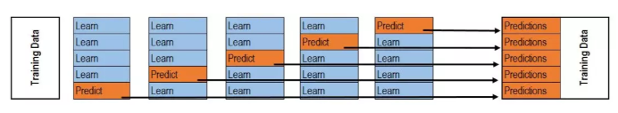
- 利用K折交叉验证(初级模型)
K-折交叉验证: 训练:
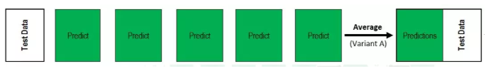
预测:
5.4 代码示例
5.4.1 回归\分类概率-融合:
1)简单加权平均,结果直接融合(不经过另一个模型预测)
## 生成一些简单的样本数据,test_prei 代表第i个模型的预测值(根据测试集生成的预测值)test_pre1 = [1.2, 3.2, 2.1, 6.2]test_pre2 = [0.9, 3.1, 2.0, 5.9]test_pre3 = [1.1, 2.9, 2.2, 6.0]
# y_test_true 代表模型的真实值y_test_true = [1, 3, 2, 6]
import numpy as npimport pandas as pd## 定义结果的加权平均函数,权重系数之和为1def Weighted_method(test_pre1,test_pre2,test_pre3,w=[1/3,1/3,1/3]):# list直接和int值相乘,结果是将list的值复制n份,list不能和float相乘;Series和int/float值相乘,结果是将Series的值与int/float分别相乘
Weighted_result = w[0]*pd.Series(test_pre1)+w[1]*pd.Series(test_pre2)+w[2]*pd.Series(test_pre3)return Weighted_result
from sklearn import metrics# 各模型的预测结果计算MAEprint('Pred1 MAE:',metrics.mean_absolute_error(y_test_true, test_pre1))print('Pred2 MAE:',metrics.mean_absolute_error(y_test_true, test_pre2))print('Pred3 MAE:',metrics.mean_absolute_error(y_test_true, test_pre3))
Pred1 MAE: 0.1750000000000001

Pred2 MAE: 0.07499999999999993

Pred3 MAE: 0.10000000000000009
## 根据加权计算MAEw = [0.3,0.4,0.3] # 定义比重权值Weighted_pre = Weighted_method(test_pre1,test_pre2,test_pre3,w)print('Weighted_pre MAE:',metrics.mean_absolute_error(y_test_true, Weighted_pre))
Weighted_pre MAE: 0.05750000000000027
可以发现加权结果相对于之前的结果是有提升的,这种我们称其为简单的加权平均。
还有一些特殊的形式,比如mean平均,median平均
## 定义结果的平均值函数def Mean_method(test_pre1,test_pre2,test_pre3):# pd.Series(test_pre1)的shape为(4,),经过pd.concat(,axis=1),可理解为扩充shape里的第1维,扩充后shape为(4,3);之后再经过mean(axis=1),可理解为在shape里的第1维上球平均,平均后的shape为(4,)。这个函数也可以直接用下面这个代替:
Mean_result = (pd.Series(test_pre1) + pd.Series(test_pre2) + pd.Series(test_pre3)) / 3
Mean_result = pd.concat([pd.Series(test_pre1),pd.Series(test_pre2),pd.Series(test_pre3)],axis=1).mean(axis=1)return Mean_resultMean_pre = Mean_method(test_pre1,test_pre2,test_pre3)print('Mean_pre MAE:',metrics.mean_absolute_error(y_test_true, Mean_pre))
Mean_pre MAE: 0.06666666666666693
## 定义结果的加权中值函数def Median_method(test_pre1,test_pre2,test_pre3):Median_result = pd.concat([pd.Series(test_pre1),pd.Series(test_pre2),pd.Series(test_pre3)],axis=1).median(axis=1)return Median_resultMedian_pre = Median_method(test_pre1,test_pre2,test_pre3)print('Median_pre MAE:',metrics.mean_absolute_error(y_test_true, Median_pre))
Median_pre MAE: 0.07500000000000007
2) Stacking融合(回归):
from sklearn import linear_modeldef Stacking_method(train_reg1,train_reg2,train_reg3,y_train_true,test_pre1,test_pre2,test_pre3,model_L2= linear_model.LinearRegression()):# 元模型基于训练集预测和训练集标签进行拟合 model_L2.fit(pd.concat([pd.Series(train_reg1),pd.Series(train_reg2),pd.Series(train_reg3)],axis=1).values,y_train_true)# 元模型基于基模型的测试集预测结果进行预测
Stacking_result = model_L2.predict(pd.concat([pd.Series(test_pre1),pd.Series(test_pre2),pd.Series(test_pre3)],axis=1).values)return Stacking_result## 生成一些简单的样本数据,train_regi代表第i个模型基于训练集的预测值train_reg1 = [3.2, 8.2, 9.1, 5.2]train_reg2 = [2.9, 8.1, 9.0, 4.9]train_reg3 = [3.1, 7.9, 9.2, 5.0]# y_train_true 代表训练集的真实值,test_prei 代表第i个模型基于测试集的预测值y_train_true = [3, 8, 9, 5]test_pre1 = [1.2, 3.2, 2.1, 6.2]test_pre2 = [0.9, 3.1, 2.0, 5.9]test_pre3 = [1.1, 2.9, 2.2, 6.0]# y_test_true 代表测试集的真实值y_test_true = [1, 3, 2, 6]model_L2= linear_model.LinearRegression() # 元模型Stacking_pre = Stacking_method(train_reg1,train_reg2,train_reg3,y_train_true,test_pre1,test_pre2,test_pre3,model_L2)# 计算模型最终预测结果和测试集真实标签的MAE
print('Stacking_pre MAE:',metrics.mean_absolute_error(y_test_true, Stacking_pre))
Stacking_pre MAE: 0.04213483146067476
可以发现模型结果相对于之前有进一步的提升(简单加权平均的MAE是0.0575),这时我们需要注意的一点是,对于第二层Stacking的模型不宜选取的过于复杂,这样会导致模型在训练集上过拟合,从而使得在测试集上并不能达到很好的效果。
5.4.2 分类模型融合:
对于分类,同样的可以使用融合方法,比如简单投票,Stacking...
from sklearn.datasets import make_blobsfrom sklearn import datasetsfrom sklearn.tree import DecisionTreeClassifierimport numpy as npfrom sklearn.ensemble import RandomForestClassifierfrom sklearn.ensemble import VotingClassifierfrom xgboost import XGBClassifierfrom sklearn.linear_model import LogisticRegressionfrom sklearn.svm import SVCfrom sklearn.model_selection import train_test_splitfrom sklearn.datasets import make_moonsfrom sklearn.metrics import accuracy_score,roc_auc_scorefrom sklearn.model_selection import cross_val_scorefrom sklearn.model_selection import StratifiedKFold/opt/conda/lib/python3.6/site-packages/sklearn/ensemble/weight_boosting.py:29: DeprecationWarning: numpy.core.umath_tests is an internal NumPy module and should not be imported. It will be removed in a future NumPy release. from numpy.core.umath_tests import inner1d
1)Voting投票机制:
Voting即投票机制,分为软投票和硬投票两种,其原理采用少数服从多数的思想。
'''
硬投票:对多个模型直接进行投票,不区分模型结果的相对重要度,最终投票数最多的类为最终被预测的类。
'''
iris = datasets.load_iris()x=iris.datay=iris.targetx_train,x_test,y_train,y_test=train_test_split(x,y,test_size=0.3)# learning_rate=0.1:学习率0.1,n_estimators=150:决策树数量150,
max_depth=3:树最大深度3,min_child_weight=2:最小叶子节点权重2,
subsample=0.7:训练一课数时使用70%的样本,
colsample_bytree=0.6:训练一颗数时随机选取60%的特征,
objective='binary:logistic':目标函数:二分类——概率
clf1 = XGBClassifier(learning_rate=0.1, n_estimators=150, max_depth=3, min_child_weight=2, subsample=0.7,colsample_bytree=0.6, objective='binary:logistic')# n_estimators=50:决策树数量,min_samples_split=4:内部节点最小分裂样本数, min_samples_leaf=63:叶节点所需最小样本数,oob_score=True:使用袋外数据进行测试 clf2 = RandomForestClassifier(n_estimators=50, max_depth=1, min_samples_split=4,min_samples_leaf=63,oob_score=True)# C=0.1:正则化系数 clf3 = SVC(C=0.1)# 硬投票eclf = VotingClassifier(estimators=[('xgb', clf1), ('rf', clf2), ('svc', clf3)], voting='hard')# 将实例化的模型和标签打包成元组,并通过交叉验证逐个训练和评估正确率
# 如果大多数基模型性能较差,会拉低性能较高基模型的表现
for clf, label in zip([clf1, clf2, clf3, eclf], ['XGBBoosting', 'Random Forest', 'SVM', 'Ensemble']):scores = cross_val_score(clf, x, y, cv=5, scoring='accuracy')print("Accuracy: %0.2f (+/- %0.2f) [%s]" % (scores.mean(), scores.std(), label))
/opt/conda/lib/python3.6/site-packages/sklearn/preprocessing/label.py:151: DeprecationWarning: The truth value of an empty array is ambiguous. Returning False, but in future this will result in an error. Use `array.size > 0` to check that an array is not empty.

  if diff:

/opt/conda/lib/python3.6/site-packages/sklearn/preprocessing/label.py:151: DeprecationWarning: The truth value of an empty array is ambiguous. Returning False, but in future this will result in an error. Use `array.size > 0` to check that an array is not empty.

  if diff:

/opt/conda/lib/python3.6/site-packages/sklearn/preprocessing/label.py:151: DeprecationWarning: The truth value of an empty array is ambiguous. Returning False, but in future this will result in an error. Use `array.size > 0` to check that an array is not empty.

  if diff:

/opt/conda/lib/python3.6/site-packages/sklearn/preprocessing/label.py:151: DeprecationWarning: The truth value of an empty array is ambiguous. Returning False, but in future this will result in an error. Use `array.size > 0` to check that an array is not empty.

  if diff:

/opt/conda/lib/python3.6/site-packages/sklearn/preprocessing/label.py:151: DeprecationWarning: The truth value of an empty array is ambiguous. Returning False, but in future this will result in an error. Use `array.size > 0` to check that an array is not empty.

  if diff:
Accuracy: 0.95 (+/- 0.03) [XGBBoosting]

Accuracy: 0.33 (+/- 0.00) [Random Forest]

Accuracy: 0.95 (+/- 0.03) [SVM]
/opt/conda/lib/python3.6/site-packages/sklearn/preprocessing/label.py:151: DeprecationWarning: The truth value of an empty array is ambiguous. Returning False, but in future this will result in an error. Use `array.size > 0` to check that an array is not empty.

  if diff:

/opt/conda/lib/python3.6/site-packages/sklearn/preprocessing/label.py:151: DeprecationWarning: The truth value of an empty array is ambiguous. Returning False, but in future this will result in an error. Use `array.size > 0` to check that an array is not empty.

  if diff:

/opt/conda/lib/python3.6/site-packages/sklearn/preprocessing/label.py:151: DeprecationWarning: The truth value of an empty array is ambiguous. Returning False, but in future this will result in an error. Use `array.size > 0` to check that an array is not empty.

  if diff:

/opt/conda/lib/python3.6/site-packages/sklearn/preprocessing/label.py:151: DeprecationWarning: The truth value of an empty array is ambiguous. Returning False, but in future this will result in an error. Use `array.size > 0` to check that an array is not empty.

  if diff:

/opt/conda/lib/python3.6/site-packages/sklearn/preprocessing/label.py:151: DeprecationWarning: The truth value of an empty array is ambiguous. Returning False, but in future this will result in an error. Use `array.size > 0` to check that an array is not empty.

  if diff:

/opt/conda/lib/python3.6/site-packages/sklearn/preprocessing/label.py:151: DeprecationWarning: The truth value of an empty array is ambiguous. Returning False, but in future this will result in an error. Use `array.size > 0` to check that an array is not empty.

  if diff:

/opt/conda/lib/python3.6/site-packages/sklearn/preprocessing/label.py:151: DeprecationWarning: The truth value of an empty array is ambiguous. Returning False, but in future this will result in an error. Use `array.size > 0` to check that an array is not empty.

  if diff:

/opt/conda/lib/python3.6/site-packages/sklearn/preprocessing/label.py:151: DeprecationWarning: The truth value of an empty array is ambiguous. Returning False, but in future this will result in an error. Use `array.size > 0` to check that an array is not empty.

  if diff:
Accuracy: 0.95 (+/- 0.03) [Ensemble]
/opt/conda/lib/python3.6/site-packages/sklearn/preprocessing/label.py:151: DeprecationWarning: The truth value of an empty array is ambiguous. Returning False, but in future this will result in an error. Use `array.size > 0` to check that an array is not empty.

  if diff:

/opt/conda/lib/python3.6/site-packages/sklearn/preprocessing/label.py:151: DeprecationWarning: The truth value of an empty array is ambiguous. Returning False, but in future this will result in an error. Use `array.size > 0` to check that an array is not empty.

  if diff:
'''
软投票:和硬投票原理相同,增加了设置权重的功能,可以为不同模型设置不同权重,进而区别模型不同的重要度。
'''
x=iris.datay=iris.targetx_train,x_test,y_train,y_test=train_test_split(x,y,test_size=0.3)clf1 = XGBClassifier(learning_rate=0.1, n_estimators=150, max_depth=3, min_child_weight=2, subsample=0.8,colsample_bytree=0.8, objective='binary:logistic')clf2 = RandomForestClassifier(n_estimators=50, max_depth=1, min_samples_split=4,min_samples_leaf=63,oob_score=True)clf3 = SVC(C=0.1, probability=True)# 软投票,增加了权重参数weights,weights里增加了XGB模型的权重eclf = VotingClassifier(estimators=[('xgb', clf1), ('rf', clf2), ('svc', clf3)], voting='soft', weights=[2, 1, 1])clf1.fit(x_train, y_train)for clf, label in zip([clf1, clf2, clf3, eclf], ['XGBBoosting', 'Random Forest', 'SVM', 'Ensemble']):scores = cross_val_score(clf, x, y, cv=5, scoring='accuracy')print("Accuracy: %0.2f (+/- %0.2f) [%s]" % (scores.mean(), scores.std(), label))
/opt/conda/lib/python3.6/site-packages/sklearn/preprocessing/label.py:151: DeprecationWarning: The truth value of an empty array is ambiguous. Returning False, but in future this will result in an error. Use `array.size > 0` to check that an array is not empty.

  if diff:

/opt/conda/lib/python3.6/site-packages/sklearn/preprocessing/label.py:151: DeprecationWarning: The truth value of an empty array is ambiguous. Returning False, but in future this will result in an error. Use `array.size > 0` to check that an array is not empty.

  if diff:

/opt/conda/lib/python3.6/site-packages/sklearn/preprocessing/label.py:151: DeprecationWarning: The truth value of an empty array is ambiguous. Returning False, but in future this will result in an error. Use `array.size > 0` to check that an array is not empty.

  if diff:

/opt/conda/lib/python3.6/site-packages/sklearn/preprocessing/label.py:151: DeprecationWarning: The truth value of an empty array is ambiguous. Returning False, but in future this will result in an error. Use `array.size > 0` to check that an array is not empty.

  if diff:

/opt/conda/lib/python3.6/site-packages/sklearn/preprocessing/label.py:151: DeprecationWarning: The truth value of an empty array is ambiguous. Returning False, but in future this will result in an error. Use `array.size > 0` to check that an array is not empty.

  if diff:
Accuracy: 0.96 (+/- 0.02) [XGBBoosting]

Accuracy: 0.33 (+/- 0.00) [Random Forest]

Accuracy: 0.95 (+/- 0.03) [SVM]
/opt/conda/lib/python3.6/site-packages/sklearn/preprocessing/label.py:151: DeprecationWarning: The truth value of an empty array is ambiguous. Returning False, but in future this will result in an error. Use `array.size > 0` to check that an array is not empty.

  if diff:

/opt/conda/lib/python3.6/site-packages/sklearn/preprocessing/label.py:151: DeprecationWarning: The truth value of an empty array is ambiguous. Returning False, but in future this will result in an error. Use `array.size > 0` to check that an array is not empty.

  if diff:

/opt/conda/lib/python3.6/site-packages/sklearn/preprocessing/label.py:151: DeprecationWarning: The truth value of an empty array is ambiguous. Returning False, but in future this will result in an error. Use `array.size > 0` to check that an array is not empty.

  if diff:

/opt/conda/lib/python3.6/site-packages/sklearn/preprocessing/label.py:151: DeprecationWarning: The truth value of an empty array is ambiguous. Returning False, but in future this will result in an error. Use `array.size > 0` to check that an array is not empty.

  if diff:
Accuracy: 0.96 (+/- 0.02) [Ensemble]
/opt/conda/lib/python3.6/site-packages/sklearn/preprocessing/label.py:151: DeprecationWarning: The truth value of an empty array is ambiguous. Returning False, but in future this will result in an error. Use `array.size > 0` to check that an array is not empty.

  if diff:
2)分类的Stacking\Blending融合:
stacking是一种分层模型集成框架。
以两层为例,第一层由多个基学习器组成,其输入为原始训练集,第二层的模型则是以第一层基学习器的输出作为训练集进行再训练,从而得到完整的stacking模型, stacking两层模型都使用了全部的训练数据。
'''
5-Fold Stacking
'''
from sklearn.ensemble import RandomForestClassifierfrom sklearn.ensemble import ExtraTreesClassifier,GradientBoostingClassifierimport pandas as pd#创建训练的数据集data_0 = iris.datadata = data_0[:100,:]target_0 = iris.targettarget = target_0[:100] # 前100个标签里只有0和1,既二分类#模型融合中使用到的各个单模型clfs = [LogisticRegression(solver='lbfgs'), # 使用拟牛顿法对损失函数进行优化# 使用gini指数分裂节点
RandomForestClassifier(n_estimators=5, n_jobs=-1, criterion='gini'),# ExtraTreesClassifier使用所有样本分裂,RandomForestClassifier使用随机样本
ExtraTreesClassifier(n_estimators=5, n_jobs=-1, criterion='gini'),# 使用信息熵分裂节点
ExtraTreesClassifier(n_estimators=5, n_jobs=-1, criterion='entropy'),# subsample=0.5——使用50%的数据进行子采样训练
GradientBoostingClassifier(learning_rate=0.05, subsample=0.5, max_depth=6, n_estimators=5)]#切分一部分数据作为测试集X, X_predict, y, y_predict = train_test_split(data, target, test_size=0.3, random_state=2020)# 用训练集数量和模型数量创建全0矩阵
dataset_blend_train = np.zeros((X.shape[0], len(clfs))) # (70, 5)dataset_blend_test = np.zeros((X_predict.shape[0], len(clfs))) # (30, 5)#5折stackingn_splits = 5skf = StratifiedKFold(n_splits)skf = skf.split(X, y) # 将训练集按原始标签中各类别的比例分成5折,每折的比例一致,划分结果为样本的索引值for j, clf in enumerate(clfs):#依次训练各个单模型# 用测试集样本的数量和stacking的折数,创建一个全0矩阵,用于存放各模型在测试集上预测标签1的概率
dataset_blend_test_j = np.zeros((X_predict.shape[0], 5)) # (30,5)for i, (train, test) in enumerate(skf):#5-Fold交叉训练,使用第i个部分作为预测,剩余的部分来训练模型,获得其预测的输出作为第i部分的新特征。# train和test为每折训练集、测试集索引
X_train, y_train, X_test, y_test = X[train], y[train], X[test], y[test]clf.fit(X_train, y_train)y_submission = clf.predict_proba(X_test)[:, 1] # 取每个训练样本被预测为标签1的概率,并作为第二层模型的特征dataset_blend_train[test, j] = y_submission # 按Fold中划分为测试集的索引,更新全0矩阵为预测标签1的概率,5轮过后,模型j基于训练集的的预测结果准备完备dataset_blend_test_j[:, i] = clf.predict_proba(X_predict)[:, 1] # 在测试集上进行预测,并将每一轮预测结果中标签1的概率保存在全0矩阵#对于测试集,直接用这k个模型的预测值均值(K折)作为新的特征。dataset_blend_test[:, j] = dataset_blend_test_j.mean(1)# y_predict为测试集真实标签,dataset_blend_test为预测标签的概率
print("val auc Score: %f" % roc_auc_score(y_predict, dataset_blend_test[:, j]))clf = LogisticRegression(solver='lbfgs')clf.fit(dataset_blend_train, y) # 在训练集预测结果上训练y_submission = clf.predict_proba(dataset_blend_test)[:, 1] # 在测试集预测结果上进行预测,并取标签1的预测值,相当于预测为正类别的概率print("Val auc Score of Stacking: %f" % (roc_auc_score(y_predict, y_submission)))
val auc Score: 1.000000

val auc Score: 0.500000

val auc Score: 0.500000

val auc Score: 0.500000

val auc Score: 0.500000

Val auc Score of Stacking: 1.000000
Blending,其实和Stacking是一种类似的多层模型融合的形式
其主要思路是把原始的训练集先分成两部分,比如70%的数据作为新的训练集,剩下30%的数据作为测试集。
在第一层,我们在这70%的数据上训练多个模型,然后去预测那30%数据的label,同时也预测test集的label。
在第二层,我们就直接用这30%数据在第一层预测的结果做为新特征继续训练,然后用test集第一层预测的label做特征,用第二层训练的模型做进一步预测
其优点在于:
- 1.比stacking简单(因为不用进行k次的交叉验证来获得stacker feature)
- 2.避开了一个信息泄露问题:generlizers和stacker使用了不一样的数据集(训练集标签不一样)
缺点在于:
- 1.使用了很少的数据(第二阶段的blender只使用training set10%的量)
- 2.blender可能会过拟合
- 3.stacking使用多次的交叉验证会比较稳健
'''
Blending
'''
#创建训练的数据集data_0 = iris.datadata = data_0[:100,:]target_0 = iris.targettarget = target_0[:100]#模型融合中使用到的各个单模型clfs = [LogisticRegression(solver='lbfgs'),RandomForestClassifier(n_estimators=5, n_jobs=-1, criterion='gini'),RandomForestClassifier(n_estimators=5, n_jobs=-1, criterion='entropy'),ExtraTreesClassifier(n_estimators=5, n_jobs=-1, criterion='gini'),#ExtraTreesClassifier(n_estimators=5, n_jobs=-1, criterion='entropy'),GradientBoostingClassifier(learning_rate=0.05, subsample=0.5, max_depth=6, n_estimators=5)]#切分一部分数据作为测试集X, X_predict, y, y_predict = train_test_split(data, target, test_size=0.3, random_state=2020)#切分训练数据集为d1,d2两部分,随机划分X_d1, X_d2, y_d1, y_d2 = train_test_split(X, y, test_size=0.5, random_state=2020)dataset_d1 = np.zeros((X_d2.shape[0], len(clfs))) # (35,5)dataset_d2 = np.zeros((X_predict.shape[0], len(clfs))) # (30,5)# X_d1:训练集;X_d2:验证集;X_predict:测试集
for j, clf in enumerate(clfs): # enumerate在逐个取模型时,还保存了模型对应的编号#依次训练各个单模型clf.fit(X_d1, y_d1) # 在一半训练集上训练y_submission = clf.predict_proba(X_d2)[:, 1] # 在另一半训练集上预测dataset_d1[:, j] = y_submission # 保存各模型在一半训练集上的预测结果#对于测试集,直接用这k个模型的预测值作为新的特征。dataset_d2[:, j] = clf.predict_proba(X_predict)[:, 1] # 各模型在测试集上的预测值,取标签1的概率print("val auc Score: %f" % roc_auc_score(y_predict, dataset_d2[:, j]))#融合使用的模型clf = GradientBoostingClassifier(learning_rate=0.02, subsample=0.5, max_depth=6, n_estimators=30)clf.fit(dataset_d1, y_d2) # 使用一半训练集上的预测结果和真实标签进行训练y_submission = clf.predict_proba(dataset_d2)[:, 1]print("Val auc Score of Blending: %f" % (roc_auc_score(y_predict, y_submission)))
val auc Score: 1.000000

val auc Score: 1.000000

val auc Score: 1.000000

val auc Score: 1.000000

val auc Score: 1.000000

Val auc Score of Blending: 1.000000
参考博客:回归分析的五个基本假设_回归分析经典假设-CSDN博客
3)分类的Stacking融合(利用mlxtend):
!pip install mlxtendimport warningswarnings.filterwarnings('ignore')import itertools # 创建迭代器import numpy as npimport seaborn as snsimport matplotlib.pyplot as pltimport matplotlib.gridspec as gridspec # 指定画布中子图位置的模块from sklearn import datasetsfrom sklearn.linear_model import LogisticRegressionfrom sklearn.neighbors import KNeighborsClassifierfrom sklearn.naive_bayes import GaussianNBfrom sklearn.ensemble import RandomForestClassifierfrom mlxtend.classifier import StackingClassifierfrom sklearn.model_selection import cross_val_scorefrom mlxtend.plotting import plot_learning_curves # 绘制分类器的学习曲线from mlxtend.plotting import plot_decision_regions # 绘制分类器的决策边界# 以python自带的鸢尾花数据集为例iris = datasets.load_iris()X, y = iris.data[:, 1:3], iris.target # 只取鸢尾花1、2两个特征clf1 = KNeighborsClassifier(n_neighbors=1) # 距离最近的点数量取1clf2 = RandomForestClassifier(random_state=1) # 默认树数量为10clf3 = GaussianNB()lr = LogisticRegression()sclf = StackingClassifier(classifiers=[clf1, clf2, clf3], # 第一层模型meta_classifier=lr) # 第二层模型label = ['KNN', 'Random Forest', 'Naive Bayes', 'Stacking Classifier']clf_list = [clf1, clf2, clf3, sclf]fig = plt.figure(figsize=(10,8))gs = gridspec.GridSpec(2, 2)grid = itertools.product([0,1],repeat=2)# grid:[(0,0), (0,1), (1,0), (1,1)]
clf_cv_mean = []clf_cv_std = []for clf, label, grd in zip(clf_list, label, grid):scores = cross_val_score(clf, X, y, cv=3, scoring='accuracy')print("Accuracy: %.2f (+/- %.2f) [%s]" %(scores.mean(), scores.std(), label))clf_cv_mean.append(scores.mean())clf_cv_std.append(scores.std())clf.fit(X, y)ax = plt.subplot(gs[grd[0], grd[1]])fig = plot_decision_regions(X=X, y=y, clf=clf)plt.title(label)plt.show()
Defaulting to user installation because normal site-packages is not writeable

Looking in indexes: https://mirrors.aliyun.com/pypi/simple

Requirement already satisfied: mlxtend in /data/nas/workspace/envs/python3.6/site-packages (0.17.3)

Requirement already satisfied: scikit-learn>=0.20.3 in /opt/conda/lib/python3.6/site-packages (from mlxtend) (0.23.2)

Requirement already satisfied: pandas>=0.24.2 in /data/nas/workspace/envs/python3.6/site-packages (from mlxtend) (1.1.4)

Requirement already satisfied: matplotlib>=3.0.0 in /opt/conda/lib/python3.6/site-packages (from mlxtend) (3.3.3)

Requirement already satisfied: scipy>=1.2.1 in /opt/conda/lib/python3.6/site-packages (from mlxtend) (1.5.4)

Requirement already satisfied: numpy>=1.16.2 in /opt/conda/lib/python3.6/site-packages (from mlxtend) (1.19.1)

Requirement already satisfied: joblib>=0.13.2 in /opt/conda/lib/python3.6/site-packages (from mlxtend) (0.17.0)

Requirement already satisfied: setuptools in /opt/conda/lib/python3.6/site-packages (from mlxtend) (49.6.0)

Requirement already satisfied: threadpoolctl>=2.0.0 in /opt/conda/lib/python3.6/site-packages (from scikit-learn>=0.20.3->mlxtend) (2.1.0)

Requirement already satisfied: pytz>=2017.2 in /opt/conda/lib/python3.6/site-packages (from pandas>=0.24.2->mlxtend) (2020.4)

Requirement already satisfied: python-dateutil>=2.7.3 in /opt/conda/lib/python3.6/site-packages (from pandas>=0.24.2->mlxtend) (2.8.1)

Requirement already satisfied: pillow>=6.2.0 in /opt/conda/lib/python3.6/site-packages (from matplotlib>=3.0.0->mlxtend) (8.0.1)

Requirement already satisfied: kiwisolver>=1.0.1 in /opt/conda/lib/python3.6/site-packages (from matplotlib>=3.0.0->mlxtend) (1.2.0)

Requirement already satisfied: pyparsing!=2.0.4,!=2.1.2,!=2.1.6,>=2.0.3 in /opt/conda/lib/python3.6/site-packages (from matplotlib>=3.0.0->mlxtend) (2.4.7)

Requirement already satisfied: cycler>=0.10 in /opt/conda/lib/python3.6/site-packages (from matplotlib>=3.0.0->mlxtend) (0.10.0)

Requirement already satisfied: six>=1.5 in /opt/conda/lib/python3.6/site-packages (from python-dateutil>=2.7.3->pandas>=0.24.2->mlxtend) (1.15.0)

Accuracy: 0.91 (+/- 0.01) [KNN]

Accuracy: 0.91 (+/- 0.06) [Random Forest]

Accuracy: 0.92 (+/- 0.03) [Naive Bayes]

Accuracy: 0.95 (+/- 0.03) [Stacking Classifier]
<Figure size 1000x800 with 4 Axes>
可以发现基模型用 'KNN', 'Random Forest', 'Naive Bayes' ,然后在这基础上, 次级模型加一个 'LogisticRegression',模型测试效果有着很好的提升。
5.4.3 一些其它方法:
将特征放进模型中预测,并将预测结果变换并作为新的特征加入原有特征中再经过模型预测结果 (Stacking变化)
(可以反复预测多次将结果加入最后的特征中)
def Ensemble_add_feature(train,test,target,clfs):# n_flods = 5# skf = list(StratifiedKFold(y, n_folds=n_flods))train_ = np.zeros((train.shape[0],len(clfs*2))) # (训练样本数量, 基模型数量*2),加下划线以示和train参数的区别test_ = np.zeros((test.shape[0],len(clfs*2)))for j,clf in enumerate(clfs):'''依次训练各个单模型'''# print(j, clf)'''使用第1个部分作为预测,第2部分来训练模型,获得其预测的输出作为第2部分的新特征。'''# X_train, y_train, X_test, y_test = X[train], y[train], X[test], y[test]clf.fit(train,target) # 用训练集拟合模型y_train = clf.predict(train) # 用训练好的模型预测训练集y_test = clf.predict(test) # 预测测试集## 新特征生成train_[:,j*2] = y_train**2 # 新特征对应的列为:0、2、4、6、8,保存预测值的平方值test_[:,j*2] = y_test**2train_[:, j+1] = np.exp(y_train) # 新特征对应的列为:1、2、3、4、5,保存预测值的指数值test_[:, j+1] = np.exp(y_test)# print("val auc Score: %f" % r2_score(y_predict, dataset_d2[:, j]))print('Method ',j)train_ = pd.DataFrame(train_)test_ = pd.DataFrame(test_)return train_,test_from sklearn.model_selection import cross_val_score, train_test_splitfrom sklearn.linear_model import LogisticRegressionclf = LogisticRegression()data_0 = iris.datadata = data_0[:100,:]target_0 = iris.targettarget = target_0[:100]x_train,x_test,y_train,y_test=train_test_split(data,target,test_size=0.3)x_train = pd.DataFrame(x_train) ; x_test = pd.DataFrame(x_test)#模型融合中使用到的各个单模型clfs = [LogisticRegression(),RandomForestClassifier(n_estimators=5, n_jobs=-1, criterion='gini'),ExtraTreesClassifier(n_estimators=5, n_jobs=-1, criterion='gini'),ExtraTreesClassifier(n_estimators=5, n_jobs=-1, criterion='entropy'),GradientBoostingClassifier(learning_rate=0.05, subsample=0.5, max_depth=6, n_estimators=5)]# x_train的shape为(70, 4),New_train的shape为(70, 10),且New_train里保存的是预测值
New_train,New_test = Ensemble_add_feature(x_train,x_test,y_train,clfs)clf = LogisticRegression()# clf = GradientBoostingClassifier(learning_rate=0.02, subsample=0.5, max_depth=6, n_estimators=30)clf.fit(New_train, y_train)y_emb = clf.predict_proba(New_test)[:, 1]print("Val auc Score of stacking: %f" % (roc_auc_score(y_test, y_emb)))
Method  0

Method  1

Method  2

Method  3

Method  4

Val auc Score of stacking: 1.000000
5.4.4 本赛题示例
import pandas as pdimport numpy as npimport warningsimport matplotlibimport matplotlib.pyplot as pltimport seaborn as snswarnings.filterwarnings('ignore')%matplotlib inlineimport itertoolsimport matplotlib.gridspec as gridspecfrom sklearn import datasetsfrom sklearn.linear_model import LogisticRegressionfrom sklearn.neighbors import KNeighborsClassifierfrom sklearn.naive_bayes import GaussianNBfrom sklearn.ensemble import RandomForestClassifier# from mlxtend.classifier import StackingClassifierfrom sklearn.model_selection import cross_val_score, train_test_split# from mlxtend.plotting import plot_learning_curves# from mlxtend.plotting import plot_decision_regionsfrom sklearn.model_selection import StratifiedKFoldfrom sklearn.model_selection import train_test_splitfrom sklearn import linear_modelfrom sklearn import preprocessingfrom sklearn.svm import SVRfrom sklearn.decomposition import PCA,FastICA,FactorAnalysis,SparsePCAimport lightgbm as lgbimport xgboost as xgbfrom sklearn.model_selection import GridSearchCVfrom sklearn.ensemble import RandomForestRegressor,GradientBoostingRegressorfrom sklearn.metrics import mean_squared_error, mean_absolute_error## 数据读取#Train_data = pd.read_csv('datalab/231784/used_car_train_20200313.csv', sep=' ')#TestA_data = pd.read_csv('datalab/231784/used_car_testA_20200313.csv', sep=' ')path = './data/'## 1) 载入训练集和测试集;Train_data = pd.read_csv(path+'train.csv', sep=' ') # 默认分隔符为逗号TestA_data = pd.read_csv(path+'testA.csv', sep=' ')print(Train_data.shape)print(TestA_data.shape)
(150000, 31)

(50000, 30)
Train_data.head()
[22]:
, , , , , , , , , , , , , , , , , , , , , , , , , , , , , , , , , , , , , , , , , , , , , , , , , , , , , , , , , , , , , , , , , , , , , , , , , , , , , , , , , , , , , , , , , , , , , , , , , , , , , , , , , , , , , , , , , , , , , , , , , , , , , , , , , , , , , , , , , , , , , , , , , , , , , , ,
| SaleID | name | regDate | model | brand | bodyType | fuelType | gearbox | power | kilometer | ... | v_5 | v_6 | v_7 | v_8 | v_9 | v_10 | v_11 | v_12 | v_13 | v_14 | |
|---|---|---|---|---|---|---|---|---|---|---|---|---|---|---|---|---|---|---|---|---|---|
| 0 | 0 | 736 | 20040402 | 30.0 | 6 | 1.0 | 0.0 | 0.0 | 60 | 12.5 | ... | 0.235676 | 0.101988 | 0.129549 | 0.022816 | 0.097462 | -2.881803 | 2.804097 | -2.420821 | 0.795292 | 0.914762 |
| 1 | 1 | 2262 | 20030301 | 40.0 | 1 | 2.0 | 0.0 | 0.0 | 0 | 15.0 | ... | 0.264777 | 0.121004 | 0.135731 | 0.026597 | 0.020582 | -4.900482 | 2.096338 | -1.030483 | -1.722674 | 0.245522 |
| 2 | 2 | 14874 | 20040403 | 115.0 | 15 | 1.0 | 0.0 | 0.0 | 163 | 12.5 | ... | 0.251410 | 0.114912 | 0.165147 | 0.062173 | 0.027075 | -4.846749 | 1.803559 | 1.565330 | -0.832687 | -0.229963 |
| 3 | 3 | 71865 | 19960908 | 109.0 | 10 | 0.0 | 0.0 | 1.0 | 193 | 15.0 | ... | 0.274293 | 0.110300 | 0.121964 | 0.033395 | 0.000000 | -4.509599 | 1.285940 | -0.501868 | -2.438353 | -0.478699 |
| 4 | 4 | 111080 | 20120103 | 110.0 | 5 | 1.0 | 0.0 | 0.0 | 68 | 5.0 | ... | 0.228036 | 0.073205 | 0.091880 | 0.078819 | 0.121534 | -1.896240 | 0.910783 | 0.931110 | 2.834518 | 1.923482 |
5 rows × 31 columns
# 排除object类型特征(notRepairedDamage)
numerical_cols = Train_data.select_dtypes(exclude = 'object').columns
print(numerical_cols)
Index(['SaleID', 'name', 'regDate', 'model', 'brand', 'bodyType', 'fuelType',

       'gearbox', 'power', 'kilometer', 'regionCode', 'seller', 'offerType',

       'creatDate', 'price', 'v_0', 'v_1', 'v_2', 'v_3', 'v_4', 'v_5', 'v_6',

       'v_7', 'v_8', 'v_9', 'v_10', 'v_11', 'v_12', 'v_13', 'v_14'],

      dtype='object')
feature_cols = [col for col in numerical_cols if col not in ['SaleID','name','regDate','price']]X_data = Train_data[feature_cols]Y_data = Train_data['price']X_test = TestA_data[feature_cols]print('X train shape:',X_data.shape)print('X test shape:',X_test.shape)
X train shape: (150000, 26)

X test shape: (50000, 26)
def Sta_inf(data):print('_min',np.min(data))print('_max:',np.max(data))print('_mean',np.mean(data))print('_ptp',np.ptp(data)) # 取展平数组的最大值 - 最小值print('_std',np.std(data))print('_var',np.var(data))print('Sta of label:')Sta_inf(Y_data)
Sta of label:

_min 11

_max: 99999

_mean 5923.327333333334

_ptp 99988

_std 7501.973469876635

_var 56279605.942732885
X_data = X_data.fillna(-1)X_test = X_test.fillna(-1)def build_model_lr(x_train,y_train):reg_model = linear_model.LinearRegression()reg_model.fit(x_train,y_train)return reg_modeldef build_model_ridge(x_train,y_train):reg_model = linear_model.Ridge(alpha=0.8) #alphas=range(1,100,5)reg_model.fit(x_train,y_train)return reg_modeldef build_model_lasso(x_train,y_train):reg_model = linear_model.LassoCV()reg_model.fit(x_train,y_train)return reg_modeldef build_model_gbdt(x_train,y_train):estimator =GradientBoostingRegressor(loss='ls',subsample= 0.85,max_depth= 5,n_estimators = 100)param_grid = {'learning_rate': [0.05,0.08,0.1,0.2],}gbdt = GridSearchCV(estimator, param_grid,cv=3) # 网格交叉搜索gbdt.fit(x_train,y_train)print(gbdt.best_params_)# print(gbdt.best_estimator_ )return gbdtdef build_model_xgb(x_train,y_train):model = xgb.XGBRegressor(n_estimators=120, learning_rate=0.08, gamma=0, subsample=0.8,\colsample_bytree=0.9, max_depth=5) #, objective ='reg:squarederror'model.fit(x_train, y_train)return modeldef build_model_lgb(x_train,y_train):estimator = lgb.LGBMRegressor(num_leaves=63,n_estimators = 100)param_grid = {'learning_rate': [0.01, 0.05, 0.1],}gbm = GridSearchCV(estimator, param_grid) # 默认3折交叉验证,既cv=3gbm.fit(x_train, y_train)return gbm
2)XGBoost的五折交叉回归验证实现
## xgbxgr = xgb.XGBRegressor(n_estimators=120, learning_rate=0.1, subsample=0.8,\colsample_bytree=0.9, max_depth=7) # ,objective ='reg:squarederror'scores_train = []scores = []## 5折交叉验证方式sk=StratifiedKFold(n_splits=5,shuffle=True,random_state=0) # shuffle默认值Falsefor train_ind,val_ind in sk.split(X_data,Y_data):train_x=X_data.iloc[train_ind].values # DataFrame不能直接用list选择样本train_y=Y_data.iloc[train_ind]val_x=X_data.iloc[val_ind].valuesval_y=Y_data.iloc[val_ind]xgr.fit(train_x,train_y)pred_train_xgb=xgr.predict(train_x)pred_xgb=xgr.predict(val_x)score_train = mean_absolute_error(train_y,pred_train_xgb)scores_train.append(score_train)score = mean_absolute_error(val_y,pred_xgb)scores.append(score)print('Train mae:',np.mean(scores_train))modelprint('Val mae',np.mean(scores))
Train mae: 606.4144986921809

Val mae 692.8452506087472
3)划分数据集,并用多种方法训练和预测
## Split data with valx_train,x_val,y_train,y_val = train_test_split(X_data,Y_data,test_size=0.3)## Train and Predictprint('Predict LR...')model_lr = build_model_lr(x_train,y_train)val_lr = model_lr.predict(x_val)subA_lr = model_lr.predict(X_test)print('Predict Ridge...')model_ridge = build_model_ridge(x_train,y_train)val_ridge = model_ridge.predict(x_val)subA_ridge = model_ridge.predict(X_test)print('Predict Lasso...')model_lasso = build_model_lasso(x_train,y_train)val_lasso = model_lasso.predict(x_val)subA_lasso = model_lasso.predict(X_test)print('Predict GBDT...')model_gbdt = build_model_gbdt(x_train,y_train)val_gbdt = model_gbdt.predict(x_val)subA_gbdt = model_gbdt.predict(X_test)
Predict LR...

Predict Ridge...

Predict Lasso...

Predict GBDT...

{'learning_rate': 0.2}
一般比赛中效果最为显著的两种方法
print('predict XGB...')model_xgb = build_model_xgb(x_train,y_train)val_xgb = model_xgb.predict(x_val)subA_xgb = model_xgb.predict(X_test)print('predict lgb...')model_lgb = build_model_lgb(x_train,y_train)val_lgb = model_lgb.predict(x_val)subA_lgb = model_lgb.predict(X_test)
predict XGB...

predict lgb...
print('Sta inf of lgb:')Sta_inf(subA_lgb)
Sta inf of lgb:

_min -206.1303689646786

_max: 88794.30124085308

_mean 5923.327751751804

_ptp 89000.43160981775

_std 7364.009558245546

_var 54228636.77393176
1)加权融合
def Weighted_method(test_pre1,test_pre2,test_pre3,w=[1/3,1/3,1/3]):Weighted_result = w[0]*pd.Series(test_pre1)+w[1]*pd.Series(test_pre2)+w[2]*pd.Series(test_pre3)return Weighted_result## Init the Weightw = [0.3,0.4,0.3]## 测试验证集准确度val_pre = Weighted_method(val_lgb,val_xgb,val_gbdt,w)MAE_Weighted = mean_absolute_error(y_val,val_pre)print('MAE of Weighted of val:',MAE_Weighted)## 预测数据部分subA = Weighted_method(subA_lgb,subA_xgb,subA_gbdt,w)print('Sta inf:')Sta_inf(subA)## 生成提交文件sub = pd.DataFrame()sub['SaleID'] = X_test.indexsub['price'] = subAsub.to_csv('./sub_Weighted.csv',index=False) # index=False不导出行序号
MAE of Weighted of val: 729.4180714728839

Sta inf:

_min -304.59363595965056

_max: 89409.50142591444

_mean 5923.614541418652

_ptp 89714.09506187409

_std 7336.152414010199

_var 53819132.241587676
## 与简单的LR(线性回归)进行对比val_lr_pred = model_lr.predict(x_val)MAE_lr = mean_absolute_error(y_val,val_lr_pred)print('MAE of lr:',MAE_lr)
MAE of lr: 2609.5098547530915
2)Stacking融合
## Stacking## 第一层train_lgb_pred = model_lgb.predict(x_train)train_xgb_pred = model_xgb.predict(x_train)train_gbdt_pred = model_gbdt.predict(x_train)Strak_X_train = pd.DataFrame()Strak_X_train['Method_1'] = train_lgb_predStrak_X_train['Method_2'] = train_xgb_predStrak_X_train['Method_3'] = train_gbdt_predStrak_X_val = pd.DataFrame()Strak_X_val['Method_1'] = val_lgbStrak_X_val['Method_2'] = val_xgbStrak_X_val['Method_3'] = val_gbdtStrak_X_test = pd.DataFrame()Strak_X_test['Method_1'] = subA_lgbStrak_X_test['Method_2'] = subA_xgbStrak_X_test['Method_3'] = subA_gbdStrak_X_test.head()
[37]:
, , , , , , , , , , , , , , , , , , , , , , , , , , , , , , , , , , , , , , , , , , ,
| Method_1 | Method_2 | Method_3 | |
|---|---|---|---|
| 0 | 40372.868827 | 40049.312500 | 39435.913696 |
| 1 | 236.634474 | 293.362427 | 229.986654 |
| 2 | 6791.805307 | 7556.451660 | 7166.881906 |
| 3 | 11609.582709 | 11634.577148 | 11909.418642 |
| 4 | 544.844624 | 509.720642 | 524.479113 |
## level2-methodmodel_lr_Stacking = build_model_lr(Strak_X_train,y_train)## 训练集train_pre_Stacking = model_lr_Stacking.predict(Strak_X_train)print('MAE of Stacking-LR:',mean_absolute_error(y_train,train_pre_Stacking))## 验证集val_pre_Stacking = model_lr_Stacking.predict(Strak_X_val)print('MAE of Stacking-LR:',mean_absolute_error(y_val,val_pre_Stacking## 预测集print('Predict Stacking-LR...')subA_Stacking = model_lr_Stacking.predict(Strak_X_test)
MAE of Stacking-LR: 627.801084629464

MAE of Stacking-LR: 717.4932203294699

Predict Stacking-LR...
subA_Stacking[subA_Stacking<10]=10 ## 去除过小的预测值sub = pd.DataFrame()sub['SaleID'] = X_test.indexsub['price'] = subA_Stackingsub.to_csv('./sub_Stacking.csv',index=False)print('Sta inf:')Sta_inf(subA_Stacking)
Sta inf:

_min 10.0

_max: 89700.60923151531

_mean 5921.534953256586

_ptp 89690.60923151531

_std 7385.887156533797

_var 54551329.08905089
3.4 经验总结
比赛的融合这个问题,个人的看法来说其实涉及多个层面,也是提分和提升模型鲁棒性的一种重要方法:
-
1)结果层面的融合,这种是最常见的融合方法,其可行的融合方法也有很多,比如根据结果的得分进行加权融合,还可以做Log,exp处理等。在做结果融合的时候,有一个很重要的条件是模型结果的得分要比较近似,然后结果的差异要比较大,这样的结果融合往往有比较好的效果提升。
-
2)特征层面的融合,这个层面其实感觉不叫融合,准确说可以叫分割,很多时候如果我们用同种模型训练,可以把特征进行切分给不同的模型,然后在后面进行模型或者结果融合有时也能产生比较好的效果。
-
3)模型层面的融合,模型层面的融合可能就涉及模型的堆叠和设计,比如加Staking层,部分模型的结果作为特征输入等,这些就需要多实验和思考了,基于模型层面的融合最好不同模型类型要有一定的差异,用同种模型不同的参数的收益一般是比较小的。
Task 5-模型融合 END.
--- By: ML67
    Email: maolinw67@163.com
    PS: 华中科技大学研究生, 长期混迹Tianchi等,希望和大家多多交流。
    github: https://github.com/mlw67 (近期会做一些书籍推导和代码的整理)


 144
144


 被折叠的 条评论
为什么被折叠?
被折叠的 条评论
为什么被折叠?
 到【灌水乐园】发言


