


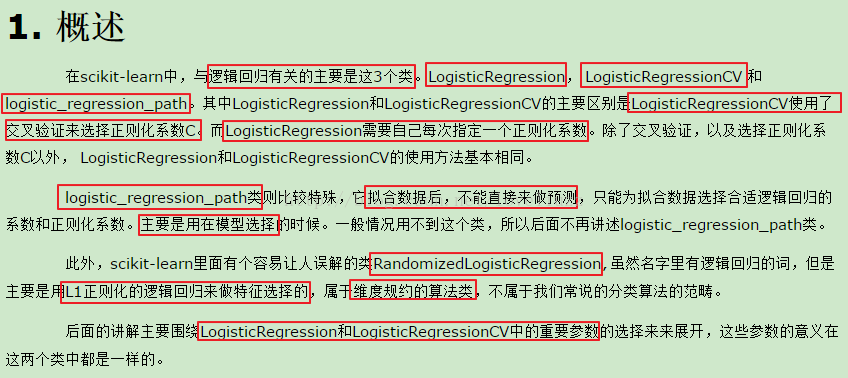
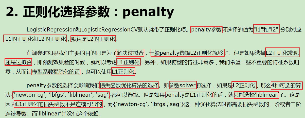
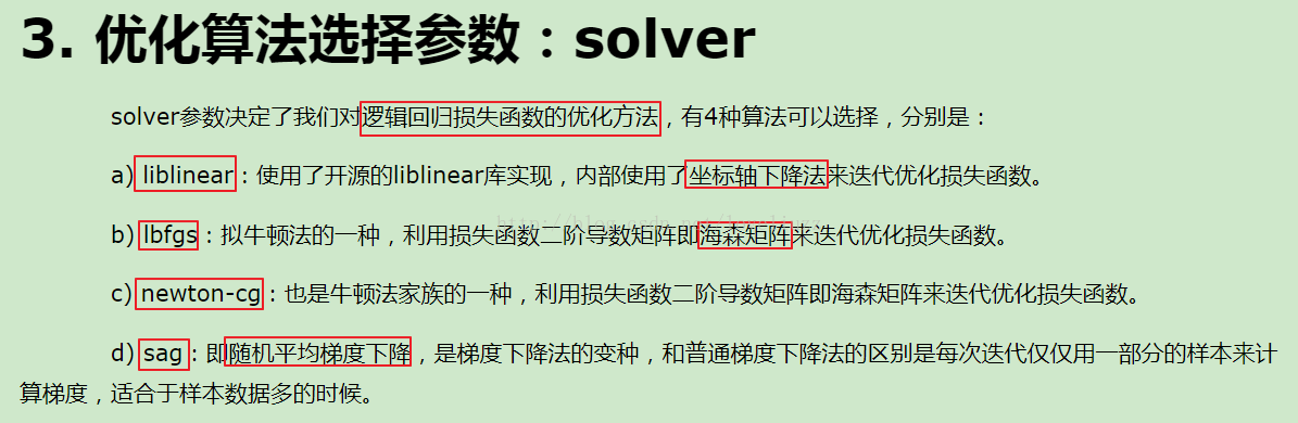
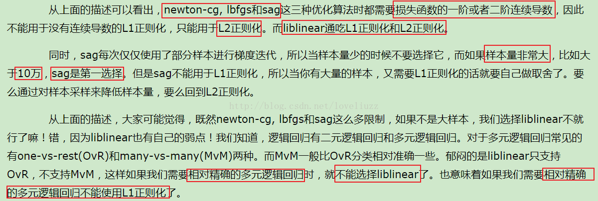
一、Logistic回归的认知与应用场景
Logistic回归为概率型非线性回归模型,是研究二分类观察结果
一种多变量分析方法。通常的问题是,研究某些因素条件下某个结果是否发生,比如医学中根据病人的一些症状
来判断它是否患有某种病。
二、LR分类器
LR分类器,即Logistic Regression Classifier。
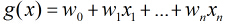
在分类情形下,经过学习后的LR分类器是一组权值
照线性加和得到 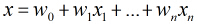


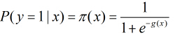
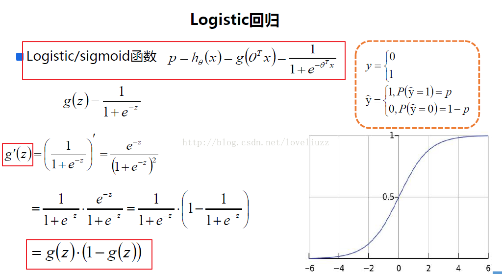
按照sigmoid函数的形式求出 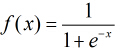

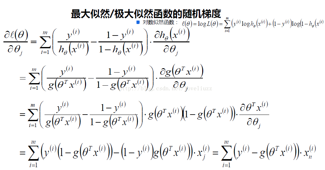
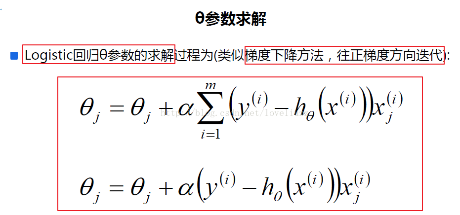
所以Logistic回归最关键的问题就是研究如何求得
三、Logistic回归模型
考虑具有
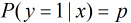
根据观测量相对于某事件
这里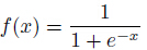
那么在
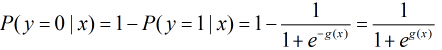
所以事件发生与不发生的概率之比为:
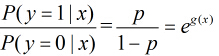
这个比值称为事件的发生比(the odds of experiencing an event),简记为odds。
小结:
一般来说,回归不用在分类问题上,因为回归是连续型模型,而且受噪声影响比较大。
如果非要应用在分类问题上,可以使用logistic回归。
logistic回归本质上是线性回归,只是在特征到结果的映射中加入了一层函数映射,
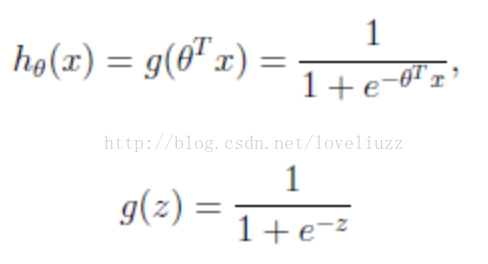
即先把特征线性求和,然后使用函数g(z)将做为假设函数来预测。g(z)可以将连续值映射到0和1上。
logistic回归的假设函数如下所示,线性回归假设函数只是![]() 。
。
logistic回归用来分类0/1问题,也就是预测结果属于0或者1的二值分类问题。
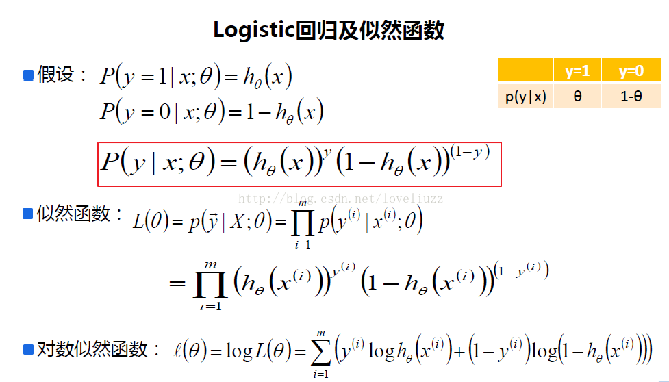
这里假设了二值满足伯努利分布(0/1分布或两点分布),也就是
四、logistic回归应用案例
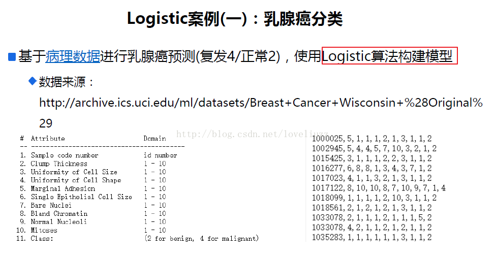
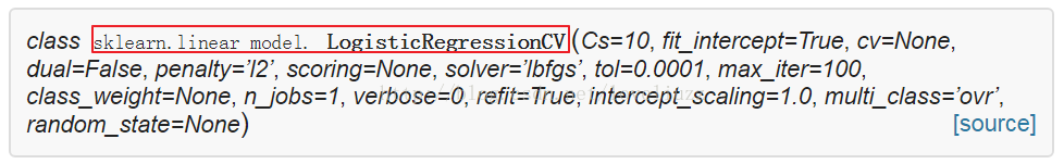
(1)sklearn中对LogisticRegressionCV函数的解析

(2)代码如下:
文件链接如下:链接:https://pan.baidu.com/s/1dEWUEhb 密码:bm1p
#!/usr/bin/env python
# -*- coding:utf-8 -*-
# Author:ZhengzhengLiu
#乳腺癌分类案例
import sklearn
from sklearn.linear_model import LogisticRegressionCV,LinearRegression
from sklearn.model_selection import train_test_split
from sklearn.preprocessing import StandardScaler
from sklearn.linear_model.coordinate_descent import ConvergenceWarning
import numpy as np
import pandas as pd
import matplotlib as mpl
import matplotlib.pyplot as plt
import warnings
#解决中文显示问题
mpl.rcParams["font.sans-serif"] = [u"SimHei"]
mpl.rcParams["axes.unicode_minus"] = False
#拦截异常
warnings.filterwarnings(action='ignore',category=ConvergenceWarning)
#导入数据并对异常数据进行清除
path = "datas/breast-cancer-wisconsin.data"
names = ["id","Clump Thickness","Uniformity of Cell Size","Uniformity of Cell Shape"
,"Marginal Adhesion","Single Epithelial Cell Size","Bare Nuclei","Bland Chromatin"
,"Normal Nucleoli","Mitoses","Class"]
df = pd.read_csv(path,header=None,names=names)
datas = df.replace("?",np.nan).dropna(how="any") #只要列中有nan值,进行行删除操作
#print(datas.head()) #默认显示前五行
#数据提取与数据分割
X = datas[names[1:10]]
Y = datas[names[10]]
#划分训练集与测试集
X_train,X_test,Y_train,Y_test = train_test_split(X,Y,test_size=0.1,random_state=0)
#对数据的训练集进行标准化
ss = StandardScaler()
X_train = ss.fit_transform(X_train) #先拟合数据在进行标准化
#构建并训练模型
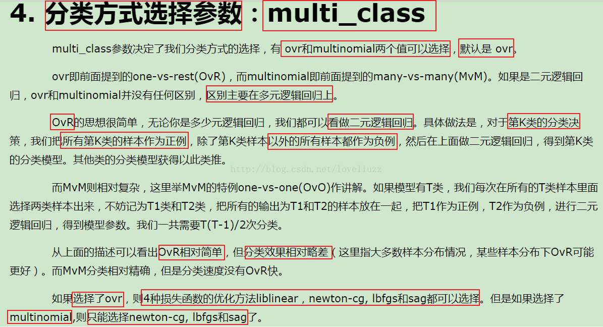
## multi_class:分类方式选择参数,有"ovr(默认)"和"multinomial"两个值可选择,在二元逻辑回归中无区别
## cv:几折交叉验证
## solver:优化算法选择参数,当penalty为"l1"时,参数只能是"liblinear(坐标轴下降法)"
## "lbfgs"和"cg"都是关于目标函数的二阶泰勒展开
## 当penalty为"l2"时,参数可以是"lbfgs(拟牛顿法)","newton_cg(牛顿法变种)","seg(minibactch随机平均梯度下降)"
## 维度<10000时,选择"lbfgs"法,维度>10000时,选择"cs"法比较好,显卡计算的时候,lbfgs"和"cs"都比"seg"快
## penalty:正则化选择参数,用于解决过拟合,可选"l1","l2"
## tol:当目标函数下降到该值是就停止,叫:容忍度,防止计算的过多
lr = LogisticRegressionCV(multi_class="ovr",fit_intercept=True,Cs=np.logspace(-2,2,20),cv=2,penalty="l2",solver="lbfgs",tol=0.01)
re = lr.fit(X_train,Y_train)
#模型效果获取
r = re.score(X_train,Y_train)
print("R值(准确率):",r)
print("参数:",re.coef_)
print("截距:",re.intercept_)
print("稀疏化特征比率:%.2f%%" %(np.mean(lr.coef_.ravel()==0)*100))
print("=========sigmoid函数转化的值,即:概率p=========")
print(re.predict_proba(X_test)) #sigmoid函数转化的值,即:概率p
#模型的保存与持久化
from sklearn.externals import joblib
joblib.dump(ss,"logistic_ss.model") #将标准化模型保存
joblib.dump(lr,"logistic_lr.model") #将训练后的线性模型保存
joblib.load("logistic_ss.model") #加载模型,会保存该model文件
joblib.load("logistic_lr.model")
#预测
X_test = ss.transform(X_test) #数据标准化
Y_predict = lr.predict(X_test) #预测
#画图对预测值和实际值进行比较
x = range(len(X_test))
plt.figure(figsize=(14,7),facecolor="w")
plt.ylim(0,6)
plt.plot(x,Y_test,"ro",markersize=8,zorder=3,label=u"真实值")
plt.plot(x,Y_predict,"go",markersize=14,zorder=2,label=u"预测值,$R^2$=%.3f" %lr.score(X_test,Y_test))
plt.legend(loc="upper left")
plt.xlabel(u"数据编号",fontsize=18)
plt.ylabel(u"乳癌类型",fontsize=18)
plt.title(u"Logistic算法对数据进行分类",fontsize=20)
plt.savefig("Logistic算法对数据进行分类.png")
plt.show()
print("=============Y_test==============")
print(Y_test.ravel())
print("============Y_predict============")
print(Y_predict)
#运行结果:
R值(准确率): 0.970684039088
参数: [[ 1.3926311 0.17397478 0.65749877 0.8929026 0.36507062 1.36092964
0.91444624 0.63198866 0.75459326]]
截距: [-1.02717163]
稀疏化特征比率:0.00%
=========sigmoid函数转化的值,即:概率p=========
[[ 6.61838068e-06 9.99993382e-01]
[ 3.78575185e-05 9.99962142e-01]
[ 2.44249065e-15 1.00000000e+00]
[ 0.00000000e+00 1.00000000e+00]
[ 1.52850624e-03 9.98471494e-01]
[ 6.67061684e-05 9.99933294e-01]
[ 6.75536843e-07 9.99999324e-01]
[ 0.00000000e+00 1.00000000e+00]
[ 2.43117004e-05 9.99975688e-01]
[ 6.13092842e-04 9.99386907e-01]
[ 0.00000000e+00 1.00000000e+00]
[ 2.00330728e-06 9.99997997e-01]
[ 0.00000000e+00 1.00000000e+00]
[ 3.78575185e-05 9.99962142e-01]
[ 4.65824155e-08 9.99999953e-01]
[ 5.47788703e-10 9.99999999e-01]
[ 0.00000000e+00 1.00000000e+00]
[ 0.00000000e+00 1.00000000e+00]
[ 0.00000000e+00 1.00000000e+00]
[ 6.27260778e-07 9.99999373e-01]
[ 3.78575185e-05 9.99962142e-01]
[ 3.85098865e-06 9.99996149e-01]
[ 1.80189197e-12 1.00000000e+00]
[ 9.44640398e-05 9.99905536e-01]
[ 0.00000000e+00 1.00000000e+00]
[ 0.00000000e+00 1.00000000e+00]
[ 4.11688915e-06 9.99995883e-01]
[ 1.85886872e-05 9.99981411e-01]
[ 5.83016713e-06 9.99994170e-01]
[ 0.00000000e+00 1.00000000e+00]
[ 1.52850624e-03 9.98471494e-01]
[ 0.00000000e+00 1.00000000e+00]
[ 0.00000000e+00 1.00000000e+00]
[ 1.51713085e-05 9.99984829e-01]
[ 2.34685008e-05 9.99976531e-01]
[ 1.51713085e-05 9.99984829e-01]
[ 0.00000000e+00 1.00000000e+00]
[ 0.00000000e+00 1.00000000e+00]
[ 2.34685008e-05 9.99976531e-01]
[ 0.00000000e+00 1.00000000e+00]
[ 9.97563915e-07 9.99999002e-01]
[ 1.70686321e-07 9.99999829e-01]
[ 1.38382134e-04 9.99861618e-01]
[ 1.36080718e-04 9.99863919e-01]
[ 1.52850624e-03 9.98471494e-01]
[ 1.68154251e-05 9.99983185e-01]
[ 6.66097483e-04 9.99333903e-01]
[ 0.00000000e+00 1.00000000e+00]
[ 9.77502258e-07 9.99999022e-01]
[ 5.83016713e-06 9.99994170e-01]
[ 0.00000000e+00 1.00000000e+00]
[ 4.09496721e-06 9.99995905e-01]
[ 0.00000000e+00 1.00000000e+00]
[ 1.37819117e-06 9.99998622e-01]
[ 6.27260778e-07 9.99999373e-01]
[ 4.52734741e-07 9.99999547e-01]
[ 0.00000000e+00 1.00000000e+00]
[ 8.88178420e-16 1.00000000e+00]
[ 1.06976766e-08 9.99999989e-01]
[ 0.00000000e+00 1.00000000e+00]
[ 2.45780192e-04 9.99754220e-01]
[ 3.92389040e-04 9.99607611e-01]
[ 6.10681985e-05 9.99938932e-01]
[ 9.44640398e-05 9.99905536e-01]
[ 1.51713085e-05 9.99984829e-01]
[ 2.45780192e-04 9.99754220e-01]
[ 2.45780192e-04 9.99754220e-01]
[ 1.51713085e-05 9.99984829e-01]
[ 0.00000000e+00 1.00000000e+00]]
=============Y_test==============
[2 2 4 4 2 2 2 4 2 2 4 2 4 2 2 2 4 4 4 2 2 2 4 2 4 4 2 2 2 4 2 4 4 2 2 2 4
4 2 4 2 2 2 2 2 2 2 4 2 2 4 2 4 2 2 2 4 2 2 4 2 2 2 2 2 2 2 2 4]
============Y_predict============
[2 2 4 4 2 2 2 4 2 2 4 2 4 2 2 2 4 4 4 2 2 2 4 2 4 4 2 2 2 4 2 4 4 2 2 2 4
4 2 4 2 2 2 2 2 2 2 4 2 2 4 2 4 2 2 2 4 4 2 4 2 2 2 2 2 2 2 2 4]五、softmax回归——多分类问题
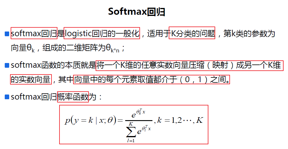
(1)softmax回归定义与概述

(2)softmax回归案例分析——葡萄酒质量预测模型
#!/usr/bin/env python
# -*- coding:utf-8 -*-
# Author:ZhengzhengLiu

#葡萄酒质量预测模型

import numpy as np
import matplotlib as mpl
import matplotlib.pyplot as plt
import pandas as pd
import warnings
import sklearn
from sklearn.linear_model import LogisticRegressionCV
from sklearn.linear_model.coordinate_descent import ConvergenceWarning
from sklearn.model_selection  import train_test_split
from sklearn.preprocessing import StandardScaler
from sklearn.preprocessing import MinMaxScaler
from sklearn.preprocessing import label_binarize
from sklearn import metrics

#解决中文显示问题
mpl.rcParams['font.sans-serif']=[u'simHei']
mpl.rcParams['axes.unicode_minus']=False

#拦截异常
warnings.filterwarnings(action = 'ignore', category=ConvergenceWarning)

#导入数据
path1 = "datas/winequality-red.csv"
df1 = pd.read_csv(path1, sep=";")
df1['type'] = 1

path2 = "datas/winequality-white.csv"
df2 = pd.read_csv(path2, sep=";")
df2['type'] = 2

df = pd.concat([df1,df2], axis=0)

names = ["fixed acidity","volatile acidity","citric acid",
         "residual sugar","chlorides","free sulfur dioxide",
         "total sulfur dioxide","density","pH","sulphates",
         "alcohol", "type"]
quality = "quality"
#print(df.head(5))

#对异常数据进行清除
new_df = df.replace('?', np.nan)
datas = new_df.dropna(how = 'any')
print ("原始数据条数:%d;异常数据处理后数据条数:%d;异常数据条数:%d" % (len(df), len(datas), len(df) - len(datas)))

#数据提取与数据分割
X = datas[names]
Y = datas[quality]

#划分训练集与测试集
X_train,X_test,Y_train,Y_test = train_test_split(X,Y,test_size=0.25,random_state=0)
print ("训练数据条数:%d;数据特征个数:%d;测试数据条数:%d" % (X_train.shape[0], X_train.shape[1], X_test.shape[0]))

#对数据的训练集进行标准化
mms = MinMaxScaler()
X_train = mms.fit_transform(X_train)

#构建并训练模型
lr = LogisticRegressionCV(fit_intercept=True, Cs=np.logspace(-5, 1, 100),
                          multi_class='multinomial', penalty='l2', solver='lbfgs')
lr.fit(X_train, Y_train)

##模型效果获取
r = lr.score(X_train, Y_train)
print ("R值:", r)
print ("特征稀疏化比率:%.2f%%" % (np.mean(lr.coef_.ravel() == 0) * 100))
print ("参数:",lr.coef_)
print ("截距:",lr.intercept_)

#预测
X_test = mms.transform(X_test)
Y_predict = lr.predict(X_test)

#画图对预测值和实际值进行比较
x_len = range(len(X_test))
plt.figure(figsize=(14,7), facecolor='w')
plt.ylim(-1,11)
plt.plot(x_len, Y_test, 'ro',markersize = 8, zorder=3, label=u'真实值')
plt.plot(x_len, Y_predict, 'go', markersize = 12, zorder=2, label=u'预测值,$R^2$=%.3f' % lr.score(X_train, Y_train))
plt.legend(loc = 'upper left')
plt.xlabel(u'数据编号', fontsize=18)
plt.ylabel(u'葡萄酒质量', fontsize=18)
plt.title(u'葡萄酒质量预测统计', fontsize=20)
plt.savefig("葡萄酒质量预测统计.png")
plt.show()

#运行结果:
原始数据条数:6497;异常数据处理后数据条数:6497;异常数据条数:0
训练数据条数:4872;数据特征个数:12;测试数据条数:1625
R值: 0.549466338259
特征稀疏化比率:0.00%
参数: [[ 0.97934119  2.16608604 -0.41710039 -0.49330657  0.90621136  1.44813439
   0.75463562  0.2311527   0.01015772 -0.69598672 -0.71473577 -0.2907567 ]
 [ 0.62487587  5.11612885 -0.38168837 -2.16145905  1.21149753 -3.71928146
  -1.45623362  1.34125165  0.33725355 -0.86655787 -2.7469681   2.02850838]
 [-1.73828753  1.96024965  0.48775556 -1.91223567  0.64365084 -1.67821019
   2.20322661  1.49086179 -1.36192671 -2.2337436  -5.01452059 -0.75501299]
 [-1.19975858 -2.60860814 -0.34557812  0.17579494 -0.04388969  0.81453743
  -0.28250319  0.51716692 -0.67756552  0.18480087  0.01838834 -0.71392084]
 [ 1.15641271 -4.6636028  -0.30902483  2.21225522 -2.00298042  1.66691445
  -1.02831849 -2.15017982  0.80529532  2.68270545  3.36326129 -0.73635195]
 [-0.07892353 -1.82724304  0.69405191  2.07681409 -0.6247279   1.49244742
  -0.16115782 -1.3671237   0.72694885  1.06878382  4.68718155  0.04669067]
 [ 0.25633987 -0.14301056  0.27158425  0.10213705 -0.08976172 -0.02454203
  -0.02964911 -0.06312954  0.15983679 -0.14000195  0.40739327  0.42084343]]
截距: [-2.34176729 -1.1649153   4.91027564  4.3206539   1.30164164 -2.25841567
 -4.76747291]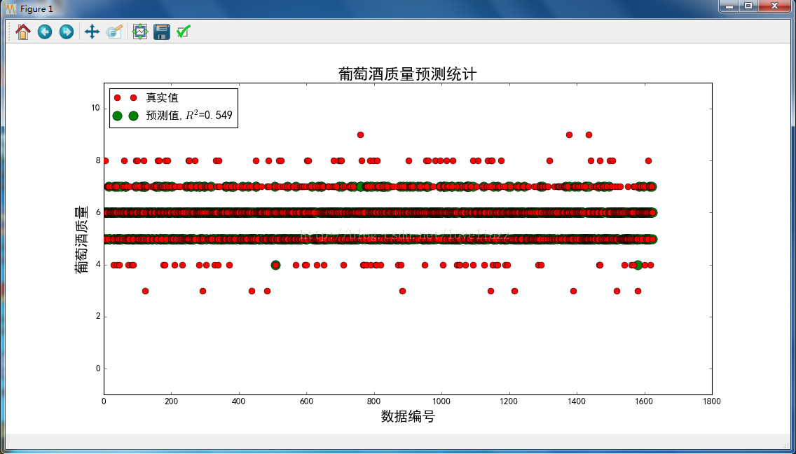
六、分类问题综合案例——鸢尾花分类问题、ROC/AUC
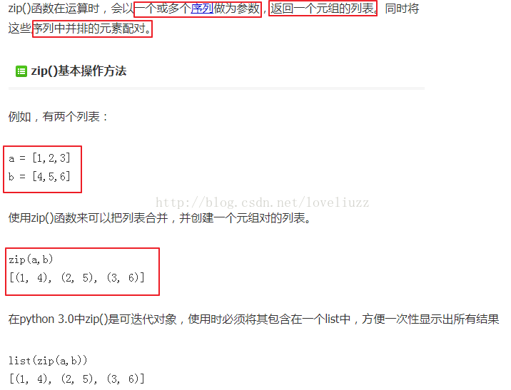
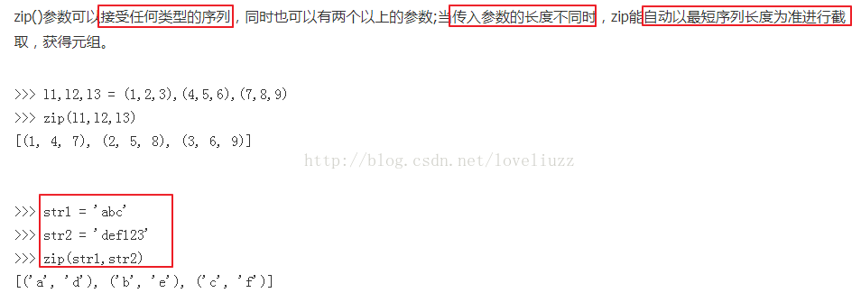
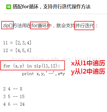
(1)知识点——python自带内置函数zip()函数
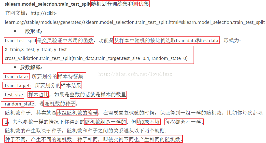
(2)知识点——sklearn.model_selection.train_test_split——随机划分训练集与测试集
(3)知识点——ROC曲线
详细链接地址:http://blog.csdn.net/abcjennifer/article/details/7359370

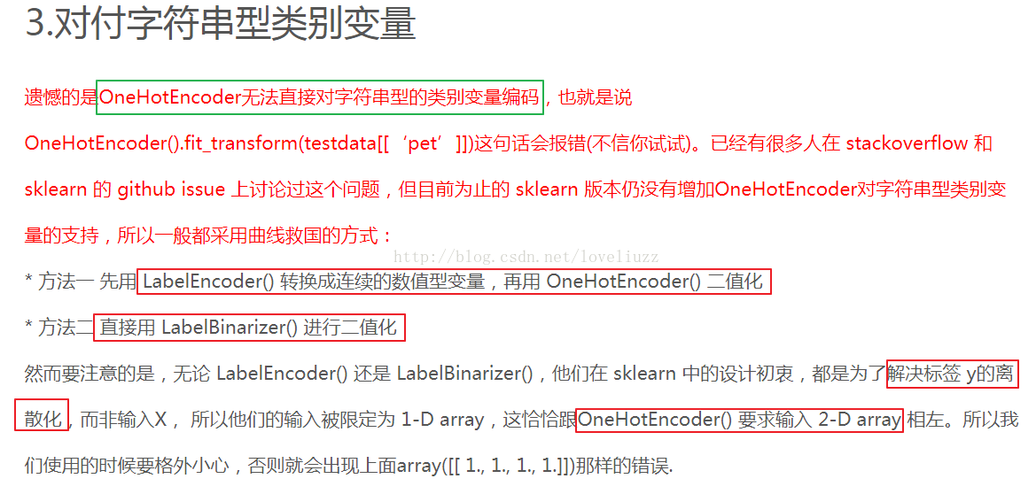
(4)知识点——所涉及到的几种 sklearn 的二值化编码函数:
OneHotEncoder(), LabelEncoder(), LabelBinarizer(), MultiLabelBinarizer()
详细链接地址为:http://blog.csdn.net/gao1440156051/article/details/55096630
案例代码:
#!/usr/bin/env python
# -*- coding:utf-8 -*-
# Author:ZhengzhengLiu
#分类综合问题——鸢尾花分类案例(ROC/AUC)
import numpy as np
import matplotlib as mpl
import matplotlib.pyplot as plt
import pandas as pd
import warnings
import sklearn
from sklearn.linear_model import LogisticRegressionCV
from sklearn.linear_model.coordinate_descent import ConvergenceWarning
from sklearn.model_selection import train_test_split
from sklearn.preprocessing import StandardScaler
from sklearn.neighbors import KNeighborsClassifier
from sklearn.preprocessing import label_binarize
from sklearn import metrics
#解决中文显示问题
mpl.rcParams['font.sans-serif']=[u'simHei']
mpl.rcParams['axes.unicode_minus']=False
#拦截异常
warnings.filterwarnings(action = 'ignore', category=ConvergenceWarning)
#导入数据
path = "datas/iris.data"
names = ['sepal length', 'sepal width', 'petal length', 'petal width', 'cla']
df = pd.read_csv(path,header=None,names=names)
print(df['cla'].value_counts())
print(df.head())
#编码函数
def parseRecord(record): #record是数据集
result = []
# zip() 函数接受一系列可迭代的对象作为参数,将对象中对应的元素按顺序组合成一个tuple,
# 每个tuple中包含的是原有序列中对应序号位置的元素,然后返回由这些tuples组成的list。
r = zip(names,record)
for name,v in r:
if name == "cla":
if v == "Iris-setosa":
result.append(1)
elif v == "Iris-versicolor":
result.append(2)
elif v == "Iris-virginica":
result.append(3)
else:
result.append(np.nan)
else:
result.append(float(v))
return result
#数据转换为数字以及分割
#数据转换
datas = df.apply(lambda r:parseRecord(r),axis=1)
print(datas.head())
#异常数据删除
datas = datas.dropna(how="any")
#数据分割
X = datas[names[0:-1]]
Y = datas[names[-1]]
#划分训练集与测试集
X_train,X_test,Y_train,Y_test = train_test_split(X,Y,test_size=0.4,random_state=0)
print("原始数据条数:%d;训练数据条数:%d;特征个数:%d;测试样本条数:%d" %(len(X),len(X_train),X_train.shape[1],len(X_test)))
#对数据集进行标准化
ss = StandardScaler()
X_train = ss.fit_transform(X_train)
X_test = ss.transform(X_test)
#构建并训练模型
lr = LogisticRegressionCV(Cs=np.logspace(-4,1,50),cv=3,fit_intercept=True,penalty="l2",
solver="lbfgs",tol=0.01,multi_class="multinomial")
lr.fit(X_train,Y_train)
#模型效果获取
#将测试集标签数据用二值化编码的方式转换为矩阵
y_test_hot = label_binarize(Y_test,classes=(1,2,3))
#得到预测的损失值
lr_y_score = lr.decision_function(X_test)
#计算ROC的值,lr_threasholds为阈值
lr_fpr,lr_tpr,lr_threasholds = metrics.roc_curve(y_test_hot.ravel(),lr_y_score.ravel())
#计算AUC值
lr_auc = metrics.auc(lr_fpr,lr_tpr)
print("Logistic算法R值:",lr.score(X_train,Y_train))
print("Logistic算法AUC值:",lr_auc)
#模型预测
lr_y_predict = lr.predict(X_test)
#画图对预测值和实际值进行比较
plt.figure(figsize=(8,6),facecolor="w")
plt.plot(lr_fpr,lr_tpr,c="r",lw=2,label=u"Logistic算法,AUC=%.3f" %lr_auc)
plt.plot((0,1),(0,1),c='#a0a0a0',lw=2,ls='--')
plt.xlim(-0.01,1.02)
plt.ylim(-0.01,1.02)
plt.xticks(np.arange(0, 1.1, 0.1))
plt.yticks(np.arange(0, 1.1, 0.1))
plt.xlabel('False Positive Rate(FPR)', fontsize=16)
plt.ylabel('True Positive Rate(TPR)', fontsize=16)
plt.grid(b=True, ls=':')
plt.legend(loc='lower right', fancybox=True, framealpha=0.8, fontsize=12)
plt.title(u'鸢尾花数据Logistic算法的ROC/AUC', fontsize=18)
plt.savefig("鸢尾花数据Logistic算法的ROC和AUC.png")
plt.show()
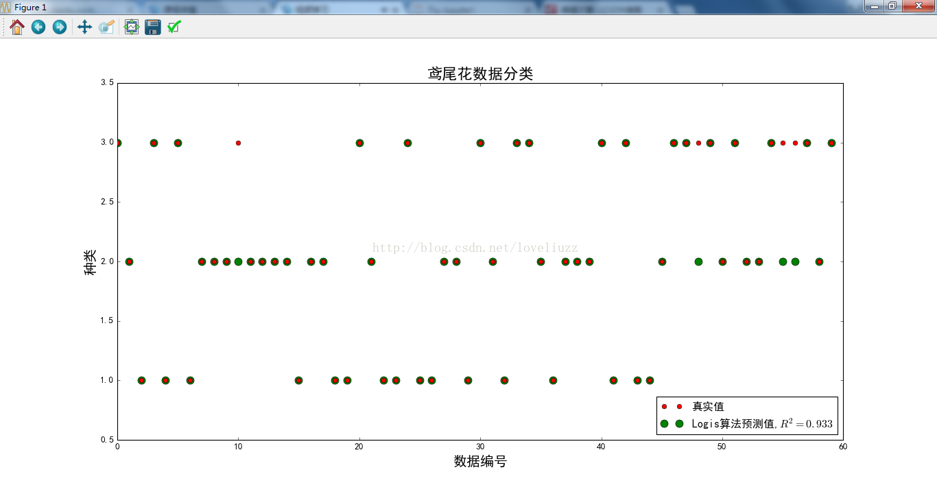
len_x_test = range(len(X_test))
plt.figure(figsize=(12,9),facecolor="w")
plt.ylim(0.5,3.5)
plt.plot(len_x_test,Y_test,"ro",markersize=6,zorder=3,label=u"真实值")
plt.plot(len_x_test,lr_y_predict,"go",markersize=10,zorder=2,label=u"Logis算法预测值,$R^2=%.3f$" %lr.score(X_test,Y_test))
plt.legend(loc = 'lower right')
plt.xlabel(u'数据编号', fontsize=18)
plt.ylabel(u'种类', fontsize=18)
plt.title(u'鸢尾花数据分类', fontsize=20)
plt.savefig("鸢尾花数据分类.png")
plt.show()
#运行结果:
Iris-versicolor 50
Iris-setosa 50
Iris-virginica 50
Name: cla, dtype: int64
sepal length sepal width petal length petal width cla
0 5.1 3.5 1.4 0.2 Iris-setosa
1 4.9 3.0 1.4 0.2 Iris-setosa
2 4.7 3.2 1.3 0.2 Iris-setosa
3 4.6 3.1 1.5 0.2 Iris-setosa
4 5.0 3.6 1.4 0.2 Iris-setosa
sepal length sepal width petal length petal width cla
0 5.1 3.5 1.4 0.2 1.0
1 4.9 3.0 1.4 0.2 1.0
2 4.7 3.2 1.3 0.2 1.0
3 4.6 3.1 1.5 0.2 1.0
4 5.0 3.6 1.4 0.2 1.0
原始数据条数:150;训练数据条数:90;特征个数:4;测试样本条数:60
Logistic算法R值: 0.977777777778
Logistic算法AUC值: 0.926944444444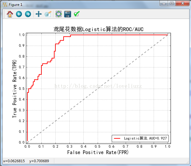


 1728
1728

 被折叠的 条评论
为什么被折叠?
被折叠的 条评论
为什么被折叠?
 到【灌水乐园】发言


