


2 正则化逻辑回归
正则化主要是解决过拟合问题,线性回归和逻辑回归均可以试用正则化处理解决过拟合问题。当训练算法在训练集表现较好,测试集上表现较差时,可能发生过拟合问题。通过合适的正则化参数lambda解决过拟合问题
2.1 作业介绍
在练习的这一部分中,您将实现规范化的逻辑回归,以预测来自制造工厂的微芯片是否通过了质量保证(QA)。在QA过程中,每个芯片都要经过各种测试,以确保其正常工作。
假设您是工厂的产品经理,您在两次不同的测试中获得了一些微芯片的测试结果。从这两个测试中,您想确定应该接受还是拒绝微芯片。为了帮助您做出决策,您有一个关于过去微芯片的测试结果的数据集,您可以从中构建一个逻辑回归模型
2.2 导入模块和数据
导入模块
import numpy as np
import matplotlib.pyplot as plt
import scipy.optimize as opt
共三列,包括前两列为测试指标,第三列是否合格
data = np.loadtxt('ex2data2.txt', delimiter=',')
print(data[:2],'\n', data.shape)
[[ 0.051267  0.69956   1.      ]
 [-0.092742  0.68494   1.      ]]
 (118, 3)
前两列赋给x,第三列赋给y
X = data[:, 0:2]
y = data[:, 2]
x样本
X[:2]
array([[ 0.051267,  0.69956 ],
       [-0.092742,  0.68494 ]])
y值,全部为0或者1,逻辑回归是分类算法,根据输入判断输出是否合格
y
array([1., 1., 1., 1., 1., 1., 1., 1., 1., 1., 1., 1., 1., 1., 1., 1., 1.,
       1., 1., 1., 1., 1., 1., 1., 1., 1., 1., 1., 1., 1., 1., 1., 1., 1.,
       1., 1., 1., 1., 1., 1., 1., 1., 1., 1., 1., 1., 1., 1., 1., 1., 1.,
       1., 1., 1., 1., 1., 1., 1., 0., 0., 0., 0., 0., 0., 0., 0., 0., 0.,
       0., 0., 0., 0., 0., 0., 0., 0., 0., 0., 0., 0., 0., 0., 0., 0., 0.,
       0., 0., 0., 0., 0., 0., 0., 0., 0., 0., 0., 0., 0., 0., 0., 0., 0.,
       0., 0., 0., 0., 0., 0., 0., 0., 0., 0., 0., 0., 0., 0., 0., 0.])
2.3 绘图函数
def plot_data(X, y):
    plt.figure()

    X0 = X[y==0]
    X1 = X[y==1]
    plt.scatter(X0[:, 0], X0[:, 1], c='r', marker='x')
    plt.scatter(X1[:, 0], X1[:, 1], c='b', marker='v')
2.4 绘图,看样本分布情况
plot_data(X, y)

plt.xlabel('Microchip Test 1')
plt.ylabel('Microchip Test 2')
plt.legend(['y = 1', 'y = 0'])

2.5 特征映射函数
通过特征映射函数将特征设成成更多维,映射后容易发生过拟合问题
def map_feature(x1, x2):
    degree = 6

    x1 = x1.reshape((x1.size, 1))
    x2 = x2.reshape((x2.size, 1))
    result = np.ones(x1[:, 0].shape)

    for i in range(1, degree + 1):
        for j in range(0, i + 1):
            result = np.c_[result, (x1**(i-j)) * (x2**j)]

    return result
给输入增加特征
X = map_feature(X[:, 0], X[:, 1])
2.6 sigmoid函数
sigmoid函数为逻辑回归激活函数,根据将输入数据将输出数据控制在0~1范围内
sigmoid公式:

def sigmoid(z):
    g = 1 / (1 + np.exp(-z))
    return g
2.7 逻辑回归代价函数和批量梯度下降(含正则化)
注:线性回归正则化部分和逻辑回归公式看起来相同,但假设函数不同
正则化代价函数公式<\b>
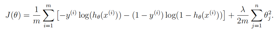
正则化逻辑回归批量梯度下降公式<\b>根据惯例正则化布包好theta0,所以批量梯度下降公式有两部分

def cost_function_reg(theta, X, y, lmd):
    m = y.size

    cost = 0
    grad = np.zeros(theta.shape)

	#逻辑回归假设函数
    hypothesis = sigmoid(np.dot(X, theta))
    #由于正则化不包含theta0,剔除theta0参数
    reg_theta = theta[1:]
    # 含正则化的代价函数
    cost = np.sum(-y * np.log(hypothesis) - (1 - y) * np.log(1 - hypothesis)) / m + (lmd / (2 * m)) * np.sum(reg_theta * reg_theta)
    # 梯度下降,不含正则化
    normal_grad = (np.dot(X.T, hypothesis - y) / m).flatten()

    grad[0] = normal_grad[0]
    #对批量题库下降除theta0外部分参数进行正则化处理
    grad[1:] = normal_grad[1:] + reg_theta * (lmd / m)

    return cost, grad
2.8 验证逻辑回归代价函数和批量梯度下降(含正则化)
初始化参数,theta全部为0
# Initialize fitting parameters 28个0
initial_theta = np.zeros(X.shape[1])

# Set regularization parameter lambda to 1
lmd = 1
# Compute and display initial cost and gradient for regularized logistic regression
cost, grad = cost_function_reg(initial_theta, X, y, lmd)

np.set_printoptions(formatter={'float': '{: 0.4f}\n'.format})
print('Cost at initial theta (zeros): {}'.format(cost))
print('Expected cost (approx): 0.693')
print('Gradient at initial theta (zeros) - first five values only: \n{}'.format(grad[0:5]))
print('Expected gradients (approx) - first five values only: \n 0.0085\n 0.0188\n 0.0001\n 0.0503\n 0.0115')
Cost at initial theta (zeros): 0.6931471805599454
Expected cost (approx): 0.693
Gradient at initial theta (zeros) - first five values only:
[ 0.0085
  0.0188
  0.0001
  0.0503
  0.0115
]
Expected gradients (approx) - first five values only:
 0.0085
 0.0188
 0.0001
 0.0503
 0.0115
测试参数全部为1时的结果
# Compute and display cost and gradient with non-zero theta
test_theta = np.ones(X.shape[1])

cost, grad = cost_function_reg(test_theta, X, y, lmd)

print('Cost at test theta: {}'.format(cost))
print('Expected cost (approx): 2.13')
print('Gradient at test theta - first five values only: \n{}'.format(grad[0:5]))
print('Expected gradients (approx) - first five values only: \n 0.3460\n 0.0851\n 0.1185\n 0.1506\n 0.0159')
Cost at test theta: 2.134848314665857
Expected cost (approx): 2.13
Gradient at test theta - first five values only:
[ 0.3460
  0.0851
  0.1185
  0.1506
  0.0159
]
Expected gradients (approx) - first five values only:
 0.3460
 0.0851
 0.1185
 0.1506
 0.0159
2.9 用高级优化方法计算代价函数和梯度
初始化参数
# Initializa fitting parameters
initial_theta = np.zeros(X.shape[1])

# Set regularization parameter lambda to 1 (you should vary this)
lmd = 1

# Optimize
def cost_func(t):
    return cost_function_reg(t, X, y, lmd)[0]
def grad_func(t):
    return cost_function_reg(t, X, y, lmd)[1]

theta, cost, *unused = opt.fmin_bfgs(f=cost_func, fprime=grad_func, x0=initial_theta, maxiter=400, full_output=True, disp=False)
2.10 Decision boundary(决策边界)函数
def plot_decision_boundary(theta, X, y):
    plot_data(X[:, 1:3], y)

    if X.shape[1] <= 3:
        # 取第一门考试成绩最大最小值坐标
        plot_x = np.array([np.min(X[:, 1]) - 2, np.max(X[:, 1]) + 2])
        # 计算决策边界线算法通过第一门考试成绩最大最小值和theta计算决策边界线的第二门考试成绩两点坐标,以便绘制决策边界线
        # 即通过两点绘制一条直线(决策边界线)
        plot_y = (-1/theta[2]) * (theta[1]*plot_x + theta[0])
        plt.plot(plot_x, plot_y)
        plt.legend(['Decision Boundary', 'Admitted', 'Not admitted'], loc=1)
        plt.axis([30, 100, 30, 100])
    else:
        # Here is the grid range
        u = np.linspace(-1, 1.5, 50)
        v = np.linspace(-1, 1.5, 50)

        z = np.zeros((u.size, v.size))

        # Evaluate z = theta*x over the grid
        for i in range(0, u.size):
            for j in range(0, v.size):
                z[i, j] = np.dot(map_feature(u[i], v[j]), theta)

        z = z.T

        # Plot z = 0
        # Notice you need to specify the range [0, 0]
        cs = plt.contour(u, v, z, levels=[0], colors='r', label='Decision Boundary')
        plt.legend([cs.collections[0]], ['Decision Boundary'])
2.11 绘制决策边界
# Plot boundary
print('Plotting decision boundary ...')
plot_decision_boundary(theta, X, y)
plt.title('lambda = {}'.format(lmd))

plt.xlabel('Microchip Test 1')
plt.ylabel('Microchip Test 2')

2.12 预测算法
假设函数


用优化后的theta根据假设函数预测样本分类:<\b>
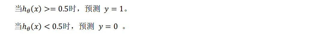
def predict(theta, X):
    m = X.shape[0]

    # Return the following variable correctly
    p = np.zeros(m)

    hypothesis = sigmoid(np.dot(X, theta))
    p = np.where(hypothesis >= 0.5, 1, 0)
#     print(p)
    # ===========================================================

    return p
预测结果,训练集训练后预测训练集准确率达83%。
正常应该将数据分成三部分:
a、训练集:不同算法训练样本
b、验证集:不同算法在验证集上验证,最小的损失值算法作为最优算法
c、测试集:用最优算法在测试集上验证
# Compute accuracy on our training set
p = predict(theta, X)

print('Train Accuracy: {:0.4f}'.format(np.mean(y == p) * 100))
print('Expected accuracy (with lambda = 1): 83.1 (approx)')
Train Accuracy: 83.0508
Expected accuracy (with lambda = 1): 83.1 (approx)


 1236
1236


 被折叠的 条评论
为什么被折叠?
被折叠的 条评论
为什么被折叠?
 到【灌水乐园】发言


