


1. 项目介绍
本项目使用 DCGAN 模型,在自建数据集上进行实验。
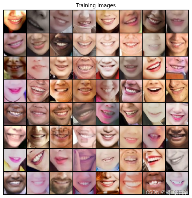
本项目使用的数据集是人脸嘴巴区域——微笑表情的数据集
数据集下载链接: https://pan.baidu.com/s/1gzoRh4gtGYC_Ucbne81BUA 提取码: tfos 复制这段内容后打开百度网盘手机App,操作更方便哦
数据集解压后文件夹结构如下,图片供 4357 张

同时,创建一个 out 文件夹来保存训练的中间结果,主要就是看 DCGAN 是如何从一张噪声照片生成我们期待的图片
import os
import time

if "out" in os.listdir("./data/"):
    print("移除现有 out 文件夹!")
    os.rmdir("./data/out")
time.sleep(1)
print("创建 out 文件夹!")
os.mkdir("./data/out")
移除现有 out 文件夹!
创建 out 文件夹!
2. 导入所需包
from __future__ import print_function
#%matplotlib inline
import argparse
import os
import random
import torch
import torch.nn as nn
import torch.nn.parallel
import torch.backends.cudnn as cudnn
import torch.optim as optim
import torch.utils.data
import torchvision.datasets as dset
import torchvision.transforms as transforms
import torchvision.utils as vutils
import numpy as np
import matplotlib.pyplot as plt
import matplotlib.animation as animation
from IPython.display import HTML

os.environ['KMP_DUPLICATE_LIB_OK'] = 'True'
3. 基本参数配置
# 设置一个随机种子,方便进行可重复性实验
manualSeed = 999
print("Random Seed: ", manualSeed)
random.seed(manualSeed)
torch.manual_seed(manualSeed)

# 数据集所在路径
dataroot = "./data/mouth/"
# 数据加载的进程数
workers = 0
# Batch size 大小
batch_size = 64
# Spatial size of training images. All images will be resized to this
# size using a transformer.
# 图片大小
image_size = 64

# 图片的通道数
nc = 3
# Size of z latent vector (i.e. size of generator input)
nz = 100
# Size of feature maps in generator
ngf = 64
# Size of feature maps in discriminator
ndf = 64
# Number of training epochs
num_epochs = 10
# Learning rate for optimizers
lr = 0.0003
# Beta1 hyperparam for Adam optimizers
beta1 = 0.5
# Number of GPUs available. Use 0 for CPU mode.
ngpu = 1

# Decide which device we want to run on
device = torch.device("cuda:0" if (torch.cuda.is_available() and ngpu > 0) else "cpu")
Random Seed: 999
4. 导入数据集
# We can use an image folder dataset the way we have it setup.
# Create the dataset
dataset = dset.ImageFolder(root=dataroot,
                           transform=transforms.Compose([
                               transforms.Resize(image_size),
                               transforms.CenterCrop(image_size),
                               transforms.ToTensor(),
                               transforms.Normalize((0.5, 0.5, 0.5), (0.5, 0.5, 0.5)),
                           ]))
# Create the dataloader
dataloader = torch.utils.data.DataLoader(dataset, batch_size=batch_size,
                                         shuffle=True, num_workers=workers)
简单看一下我们的原始数据集长啥样
# Plot some training images
real_batch = next(iter(dataloader))
plt.figure(figsize=(8,8))
plt.axis("off")
plt.title("Training Images")
plt.imshow(np.transpose(vutils.make_grid(real_batch[0].to(device)[:64], padding=2, normalize=True).cpu(),(1,2,0)))
# plt.show()
<matplotlib.image.AxesImage at 0x27012993ac0>
5. 定义生成器与判别器
# 权重初始化函数,为生成器和判别器模型初始化
def weights_init(m):
    classname = m.__class__.__name__
    if classname.find('Conv') != -1:
        nn.init.normal_(m.weight.data, 0.0, 0.02)
    elif classname.find('BatchNorm') != -1:
        nn.init.normal_(m.weight.data, 1.0, 0.02)
        nn.init.constant_(m.bias.data, 0)

# Generator Code
class Generator(nn.Module):
    def __init__(self, ngpu):
        super(Generator, self).__init__()
        self.ngpu = ngpu
        self.main = nn.Sequential(
            # input is Z, going into a convolution
            nn.ConvTranspose2d( nz, ngf * 8, 4, 1, 0, bias=False),
            nn.BatchNorm2d(ngf * 8),
            nn.ReLU(True),
            # state size. (ngf*8) x 4 x 4
            nn.ConvTranspose2d(ngf * 8, ngf * 4, 4, 2, 1, bias=False),
            nn.BatchNorm2d(ngf * 4),
            nn.ReLU(True),
            # state size. (ngf*4) x 8 x 8
            nn.ConvTranspose2d( ngf * 4, ngf * 2, 4, 2, 1, bias=False),
            nn.BatchNorm2d(ngf * 2),
            nn.ReLU(True),
            # state size. (ngf*2) x 16 x 16
            nn.ConvTranspose2d( ngf * 2, ngf, 4, 2, 1, bias=False),
            nn.BatchNorm2d(ngf),
            nn.ReLU(True),
            # state size. (ngf) x 32 x 32
            nn.ConvTranspose2d( ngf, nc, 4, 2, 1, bias=False),
            nn.Tanh()
            # state size. (nc) x 64 x 64
        )

    def forward(self, input):
        return self.main(input)


class Discriminator(nn.Module):
    def __init__(self, ngpu):
        super(Discriminator, self).__init__()
        self.ngpu = ngpu
        self.main = nn.Sequential(
            # input is (nc) x 64 x 64
            nn.Conv2d(nc, ndf, 4, 2, 1, bias=False),
            nn.LeakyReLU(0.2, inplace=True),
            # state size. (ndf) x 32 x 32
            nn.Conv2d(ndf, ndf * 2, 4, 2, 1, bias=False),
            nn.BatchNorm2d(ndf * 2),
            nn.LeakyReLU(0.2, inplace=True),
            # state size. (ndf*2) x 16 x 16
            nn.Conv2d(ndf * 2, ndf * 4, 4, 2, 1, bias=False),
            nn.BatchNorm2d(ndf * 4),
            nn.LeakyReLU(0.2, inplace=True),
            # state size. (ndf*4) x 8 x 8
            nn.Conv2d(ndf * 4, ndf * 8, 4, 2, 1, bias=False),
            nn.BatchNorm2d(ndf * 8),
            nn.LeakyReLU(0.2, inplace=True),
            # state size. (ndf*8) x 4 x 4
            nn.Conv2d(ndf * 8, 1, 4, 1, 0, bias=False),
            nn.Sigmoid()
        )

    def forward(self, input):
        return self.main(input)
6. 初始化生成器和判别器
# Create the generator
netG = Generator(ngpu).to(device)

# Handle multi-gpu if desired
if (device.type == 'cuda') and (ngpu > 1):
    netG = nn.DataParallel(netG, list(range(ngpu)))

# Apply the weights_init function to randomly initialize all weights
# to mean=0, stdev=0.2.
netG.apply(weights_init)
# Print the model
print(netG)

# Create the Discriminator
netD = Discriminator(ngpu).to(device)

# Handle multi-gpu if desired
if (device.type == 'cuda') and (ngpu > 1):
    netD = nn.DataParallel(netD, list(range(ngpu)))

# Apply the weights_init function to randomly initialize all weights
#  to mean=0, stdev=0.2.
netD.apply(weights_init)

# Print the model
print(netD)
Generator(
  (main): Sequential(
    (0): ConvTranspose2d(100, 512, kernel_size=(4, 4), stride=(1, 1), bias=False)
    (1): BatchNorm2d(512, eps=1e-05, momentum=0.1, affine=True, track_running_stats=True)
    (2): ReLU(inplace=True)
    (3): ConvTranspose2d(512, 256, kernel_size=(4, 4), stride=(2, 2), padding=(1, 1), bias=False)
    (4): BatchNorm2d(256, eps=1e-05, momentum=0.1, affine=True, track_running_stats=True)
    (5): ReLU(inplace=True)
    (6): ConvTranspose2d(256, 128, kernel_size=(4, 4), stride=(2, 2), padding=(1, 1), bias=False)
    (7): BatchNorm2d(128, eps=1e-05, momentum=0.1, affine=True, track_running_stats=True)
    (8): ReLU(inplace=True)
    (9): ConvTranspose2d(128, 64, kernel_size=(4, 4), stride=(2, 2), padding=(1, 1), bias=False)
    (10): BatchNorm2d(64, eps=1e-05, momentum=0.1, affine=True, track_running_stats=True)
    (11): ReLU(inplace=True)
    (12): ConvTranspose2d(64, 3, kernel_size=(4, 4), stride=(2, 2), padding=(1, 1), bias=False)
    (13): Tanh()
  )
)
Discriminator(
  (main): Sequential(
    (0): Conv2d(3, 64, kernel_size=(4, 4), stride=(2, 2), padding=(1, 1), bias=False)
    (1): LeakyReLU(negative_slope=0.2, inplace=True)
    (2): Conv2d(64, 128, kernel_size=(4, 4), stride=(2, 2), padding=(1, 1), bias=False)
    (3): BatchNorm2d(128, eps=1e-05, momentum=0.1, affine=True, track_running_stats=True)
    (4): LeakyReLU(negative_slope=0.2, inplace=True)
    (5): Conv2d(128, 256, kernel_size=(4, 4), stride=(2, 2), padding=(1, 1), bias=False)
    (6): BatchNorm2d(256, eps=1e-05, momentum=0.1, affine=True, track_running_stats=True)
    (7): LeakyReLU(negative_slope=0.2, inplace=True)
    (8): Conv2d(256, 512, kernel_size=(4, 4), stride=(2, 2), padding=(1, 1), bias=False)
    (9): BatchNorm2d(512, eps=1e-05, momentum=0.1, affine=True, track_running_stats=True)
    (10): LeakyReLU(negative_slope=0.2, inplace=True)
    (11): Conv2d(512, 1, kernel_size=(4, 4), stride=(1, 1), bias=False)
    (12): Sigmoid()
  )
)
7. 定义损失函数
# Initialize BCELoss function
criterion = nn.BCELoss()
8. 开始训练
# Create batch of latent vectors that we will use to visualize
#  the progression of the generator
fixed_noise = torch.randn(64, nz, 1, 1, device=device)

# Establish convention for real and fake labels during training
real_label = 1.0
fake_label = 0.0

# Setup Adam optimizers for both G and D
optimizerD = optim.Adam(netD.parameters(), lr=lr, betas=(beta1, 0.999))
optimizerG = optim.Adam(netG.parameters(), lr=lr, betas=(beta1, 0.999))

# Training Loop

# Lists to keep track of progress
img_list = []
G_losses = []
D_losses = []
iters = 0

print("Starting Training Loop...")
# For each epoch
for epoch in range(num_epochs):
    import time
    start = time.time()
    # For each batch in the dataloader
    for i, data in enumerate(dataloader, 0):

        ############################
        # (1) Update D network: maximize log(D(x)) + log(1 - D(G(z)))
        ###########################
        ## Train with all-real batch
        netD.zero_grad()
        # Format batch
        real_cpu = data[0].to(device)
        b_size = real_cpu.size(0)
        label = torch.full((b_size,), real_label, device=device)
        # Forward pass real batch through D
        output = netD(real_cpu).view(-1)
        # Calculate loss on all-real batch
        errD_real = criterion(output, label)
        # Calculate gradients for D in backward pass
        errD_real.backward()
        D_x = output.mean().item()

        ## Train with all-fake batch
        # Generate batch of latent vectors
        noise = torch.randn(b_size, nz, 1, 1, device=device)
        # Generate fake image batch with G
        fake = netG(noise)
        label.fill_(fake_label)
        # Classify all fake batch with D
        output = netD(fake.detach()).view(-1)
        # Calculate D's loss on the all-fake batch
        errD_fake = criterion(output, label)
        # Calculate the gradients for this batch
        errD_fake.backward()
        D_G_z1 = output.mean().item()
        # Add the gradients from the all-real and all-fake batches
        errD = errD_real + errD_fake
        # Update D
        optimizerD.step()

        ############################
        # (2) Update G network: maximize log(D(G(z)))
        ###########################
        netG.zero_grad()
        label.fill_(real_label)  # fake labels are real for generator cost
        # Since we just updated D, perform another forward pass of all-fake batch through D
        output = netD(fake).view(-1)
        # Calculate G's loss based on this output
        errG = criterion(output, label)
        # Calculate gradients for G
        errG.backward()
        D_G_z2 = output.mean().item()
        # Update G
        optimizerG.step()

        # Output training stats
        if i % 50 == 0:
            print('[%d/%d][%d/%d]\tLoss_D: %.4f\tLoss_G: %.4f\tD(x): %.4f\tD(G(z)): %.4f / %.4f'
                  % (epoch, num_epochs, i, len(dataloader),
                     errD.item(), errG.item(), D_x, D_G_z1, D_G_z2))

        # Save Losses for plotting later
        G_losses.append(errG.item())
        D_losses.append(errD.item())

        # Check how the generator is doing by saving G's output on fixed_noise
        if (iters % 20 == 0) or ((epoch == num_epochs-1) and (i == len(dataloader)-1)):

            with torch.no_grad():
                fake = netG(fixed_noise).detach().cpu()

            img_list.append(vutils.make_grid(fake, padding=2, normalize=True))
            i = vutils.make_grid(fake, padding=2, normalize=True)
            fig = plt.figure(figsize=(8, 8))
            plt.imshow(np.transpose(i, (1, 2, 0)))
            plt.axis('off')  # 关闭坐标轴
            plt.savefig("./data/out/%d_%d.png" % (epoch, iters))
            plt.close(fig)
        iters += 1
    print('time:', time.time() - start)
Starting Training Loop...
[0/10][0/69]	Loss_D: 1.0975	Loss_G: 4.8112	D(x): 0.6893	D(G(z)): 0.3159 / 0.0954
[0/10][50/69]	Loss_D: 0.4824	Loss_G: 4.6064	D(x): 0.8130	D(G(z)): 0.1995 / 0.0189
time: 13.753226280212402
[1/10][0/69]	Loss_D: 0.5500	Loss_G: 4.9197	D(x): 0.7818	D(G(z)): 0.1445 / 0.0235
[1/10][50/69]	Loss_D: 0.5982	Loss_G: 3.1465	D(x): 0.7039	D(G(z)): 0.1033 / 0.0676
time: 13.408677339553833
[2/10][0/69]	Loss_D: 2.3809	Loss_G: 1.1063	D(x): 0.1867	D(G(z)): 0.0156 / 0.4683
[2/10][50/69]	Loss_D: 0.8676	Loss_G: 4.0431	D(x): 0.7715	D(G(z)): 0.3795 / 0.0313
time: 14.15134596824646
[3/10][0/69]	Loss_D: 2.0267	Loss_G: 6.5130	D(x): 0.9628	D(G(z)): 0.8000 / 0.0066
[3/10][50/69]	Loss_D: 0.8248	Loss_G: 5.8990	D(x): 0.8961	D(G(z)): 0.4671 / 0.0062
time: 14.044241428375244
[4/10][0/69]	Loss_D: 1.2879	Loss_G: 5.8416	D(x): 0.9309	D(G(z)): 0.5651 / 0.0091
[4/10][50/69]	Loss_D: 0.5999	Loss_G: 3.2066	D(x): 0.6504	D(G(z)): 0.0708 / 0.0681
time: 14.462169408798218
[5/10][0/69]	Loss_D: 1.2421	Loss_G: 1.0341	D(x): 0.4554	D(G(z)): 0.1206 / 0.4578
[5/10][50/69]	Loss_D: 1.0635	Loss_G: 3.4306	D(x): 0.6589	D(G(z)): 0.3860 / 0.0539
time: 14.234107971191406
[6/10][0/69]	Loss_D: 1.6703	Loss_G: 5.9602	D(x): 0.9313	D(G(z)): 0.6313 / 0.0181
[6/10][50/69]	Loss_D: 0.5268	Loss_G: 3.0553	D(x): 0.8090	D(G(z)): 0.2370 / 0.0654
time: 14.24141526222229
[7/10][0/69]	Loss_D: 1.1129	Loss_G: 3.8517	D(x): 0.8774	D(G(z)): 0.5470 / 0.0504
[7/10][50/69]	Loss_D: 0.6979	Loss_G: 3.3661	D(x): 0.8265	D(G(z)): 0.3438 / 0.0485
time: 14.466978311538696
[8/10][0/69]	Loss_D: 3.1995	Loss_G: 4.7117	D(x): 0.9638	D(G(z)): 0.9072 / 0.0244
[8/10][50/69]	Loss_D: 0.6708	Loss_G: 3.3881	D(x): 0.8161	D(G(z)): 0.3295 / 0.0467
time: 14.965966701507568
[9/10][0/69]	Loss_D: 0.9120	Loss_G: 4.0951	D(x): 0.8086	D(G(z)): 0.4406 / 0.0276
[9/10][50/69]	Loss_D: 0.7384	Loss_G: 2.3728	D(x): 0.6775	D(G(z)): 0.2310 / 0.1272
time: 14.140359878540039
9. 绘制损失曲线
plt.figure(figsize=(10,5))
plt.title("Generator and Discriminator Loss During Training")
plt.plot(G_losses,label="G")
plt.plot(D_losses,label="D")
plt.xlabel("iterations")
plt.ylabel("Loss")
plt.legend()
plt.show()

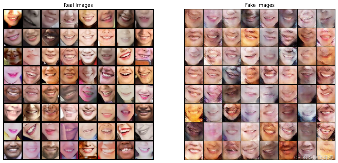
10. 真假对比
# Grab a batch of real images from the dataloader
# real_batch = next(iter(dataloader))

# Plot the real images
plt.figure(figsize=(15,15))
plt.subplot(1,2,1)
plt.axis("off")
plt.title("Real Images")
plt.imshow(np.transpose(vutils.make_grid(real_batch[0].to(device)[:64], padding=5, normalize=True).cpu(),(1,2,0)))

# Plot the fake images from the last epoch
plt.subplot(1,2,2)
plt.axis("off")
plt.title("Fake Images")
plt.imshow(np.transpose(img_list[-1],(1,2,0)))
plt.show()


 971
971


 被折叠的 条评论
为什么被折叠?
被折叠的 条评论
为什么被折叠?
 到【灌水乐园】发言


