视觉Transformer解析(附代码)

程序员丸子

于 2024-08-23 10:00:06 发布

阅读量605

点赞数 16

文章标签： transformer 深度学习人工智能语言模型 AI大模型大模型大语言模型

本文链接：https://blog.csdn.net/lyy2017175913/article/details/141454894

版权

自2017年**“注意力就是一切”**的理念问世以来，Transformer模型便迅速在自然语言处理（NLP）领域崭露头角，确立了其领先地位。到了2021年，“一张图片等于16x16个单词”的理念成功将Transformer模型引入计算机视觉任务中。自此之后，众多基于Transformer的架构纷纷涌现，应用于计算机视觉领域。

本文将详细介绍“一张图片等于16x16个单词”中阐述的Vision Transformer（ViT），包括其开源代码和对各组件的概念解释。所有代码均使用PyTorch Python包实现。

本文作为一系列深入研究Vision Transformers内部工作原理的文章之一，提供了可执行代码的Jupyter Notebook版本。系列中的其他文章还包括：Vision Transformers解析、注意力机制在Vision Transformers中的应用、Vision Transformers的位置编码解析、Tokens-to-Token Vision Transformers解析以及Vision Transformers解析系列的GitHub仓库等。

那么，什么是Vision Transformers呢？正如“注意力就是一切”所介绍的，Transformer是一种利用注意力机制作为主要学习机制的机器学习模型。它迅速成为序列到序列任务（如语言翻译）的领先技术。

**“一张图片等于16x16个单词”**成功地改进了[1]中提出的Transformer，使其能够应对图像分类任务，从而催生了Vision Transformer（ViT）。ViT与[1]中的Transformer一样，基于注意力机制。不过，与用于NLP任务的Transformer包含编码器和解码器两个注意力分支不同，ViT仅使用编码器。编码器的输出随后传递给神经网络“头”进行预测。

然而，“一张图片等于16x16个单词”中实现的ViT存在一个缺点，即其最佳性能需要在大型数据集上进行预训练。最佳模型是在专有的JFT-300M数据集上预训练的。而在较小的开源ImageNet-21k数据集上进行预训练的模型，其性能与最先进的卷积ResNet模型相当。

Tokens-to-Token ViT: Training Vision Transformers from Scratch on ImageNet则试图通过引入一种新颖的预处理方法，将输入图像转换为一系列token，从而消除这种预训练要求。有关此方法的更多信息，请查阅相关资料。在本文中，我们将重点讨论“一张图片等于16x16个单词”中实现的ViT。

针对所有自学遇到困难的同学们，我帮大家系统梳理大模型学习脉络，将这份 LLM大模型资料 分享出来：包括LLM大模型书籍、640套大模型行业报告、LLM大模型学习视频、LLM大模型学习路线、开源大模型学习教程等, 😝有需要的小伙伴，可以 扫描下方二维码领取🆓↓↓↓

👉[CSDN大礼包🎁：全网最全《LLM大模型入门+进阶学习资源包》免费分享（安全链接，放心点击）]()👈

模型解析

本文遵循《一张图片等于16x16个单词》中概述的模型结构。然而，该论文的代码并未公开发布。最近的《Tokens-to-Token ViT》中的代码可在GitHub上找到。Tokens-to-Token ViT（T2T-ViT）模型在普通ViT骨干结构前添加了一个Tokens-to-Token（T2T）模块。本文中的代码基于《Tokens-to-Token ViT》GitHub代码中的ViT组件。本文对代码进行了修改，以允许非方形输入图像，并移除了dropout层。

ViT模型的结构示意图如下所示。

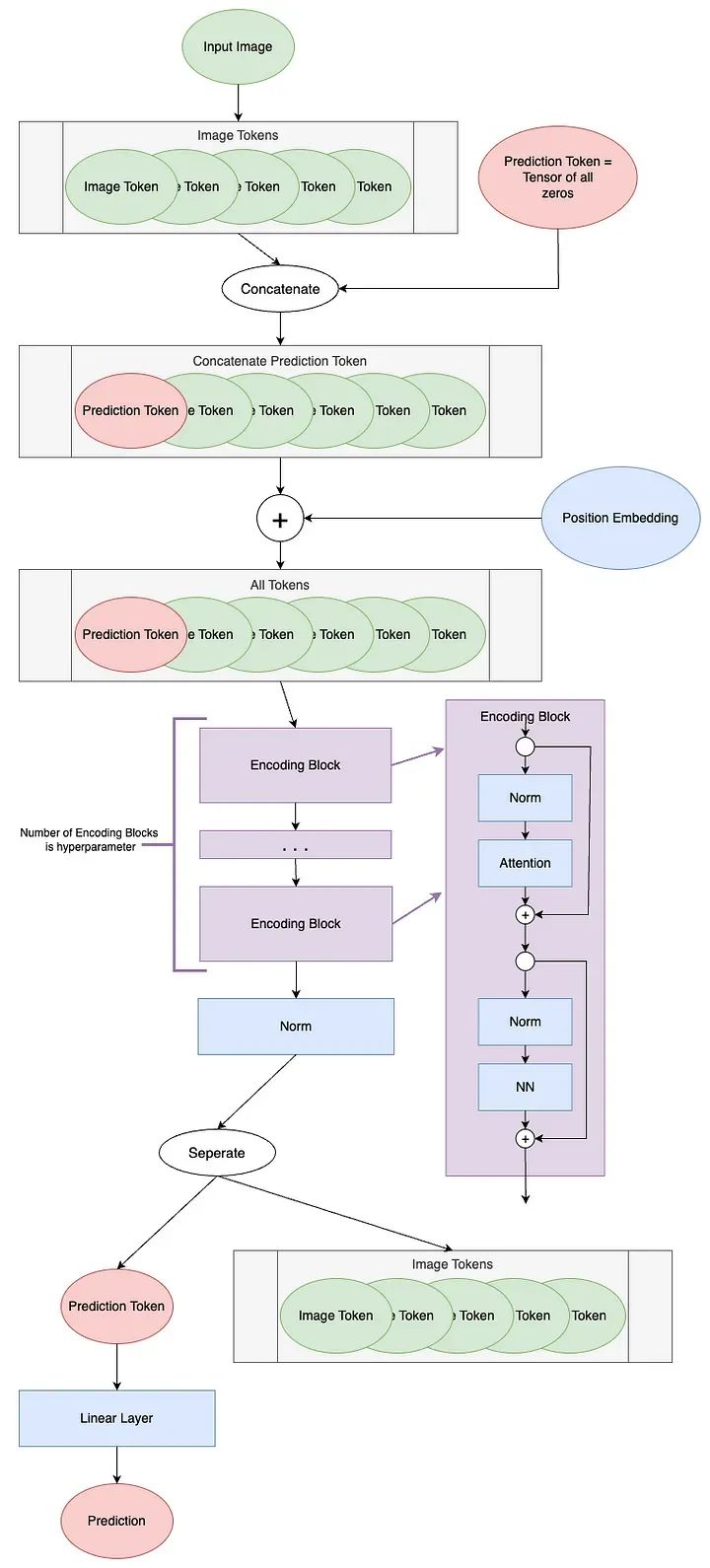
ViT模型示意图

图像Token化

ViT的第一步是从输入图像创建Token。Transformer操作的是一系列Token；在NLP中，这通常是一个句子的单词。对于计算机视觉来说，如何将输入分段成Token并不太明确。

ViT将图像转换为Token，以便每个Token表示图像的一个局部区域（或补丁）。他们描述了如何将高度H、宽度W和通道数C的图像重新塑造为N个补丁大小为P的Token：

每个Token的长度为P²*C。

让我们以此像素艺术《黄昏下的山》（作者Luis Zuno）为例进行补丁Token化。原始艺术品已被裁剪并转换为单通道图像。这意味着每个像素的值在0到1之间。单通道图像通常以灰度显示，但我们将以紫色配色方案显示它，因为这样更容易看到。请注意，补丁Token化不包括在[3]相关的代码中。

mountains = np.load(os.path.join(figure_path, 'mountains.npy'))

H = mountains.shape[0]
W = mountains.shape[1]
print('Mountain at Dusk is H =', H, 'and W =', W, 'pixels.')
print('\n')

fig = plt.figure(figsize=(10,6))
plt.imshow(mountains, cmap='Purples_r')
plt.xticks(np.arange(-0.5, W+1, 10), labels=np.arange(0, W+1, 10))
plt.yticks(np.arange(-0.5, H+1, 10), labels=np.arange(0, H+1, 10))
plt.clim([0,1])cbar_ax = fig.add_axes([0.95, .11, 0.05, 0.77])
plt.clim([0, 1])
plt.colorbar(cax=cbar_ax);
#plt.savefig(os.path.join(figure_path, 'mountains.png'))

Mountain at Dusk is H = 60 and W = 100 pixels.

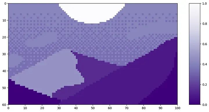
这个图像的高度为H=60，宽度为W=100。我们将设置P=20，因为它能够均匀地整除H和W。

P = 20
N = int((H*W)/(P**2))
print('There will be', N, 'patches, each', P, 'by', str(P)+'.')
print('\n')

fig = plt.figure(figsize=(10,6))
plt.imshow(mountains, cmap='Purples_r')
plt.hlines(np.arange(P, H, P)-0.5, -0.5, W-0.5, color='w')
plt.vlines(np.arange(P, W, P)-0.5, -0.5, H-0.5, color='w')
plt.xticks(np.arange(-0.5, W+1, 10), labels=np.arange(0, W+1, 10))
plt.yticks(np.arange(-0.5, H+1, 10), labels=np.arange(0, H+1, 10))
x_text = np.tile(np.arange(9.5, W, P), 3)
y_text = np.repeat(np.arange(9.5, H, P), 5)
for i in range(1, N+1):   
 plt.text(x_text[i-1], y_text[i-1], str(i), color='w', fontsize='xx-large', ha='center')
 plt.text(x_text[2], y_text[2], str(3), color='k', fontsize='xx-large', ha='center');
 #plt.savefig(os.path.join(figure_path, 'mountain_patches.png'), bbox_inches='tight'

There will be 15 patches, each 20 by 20.

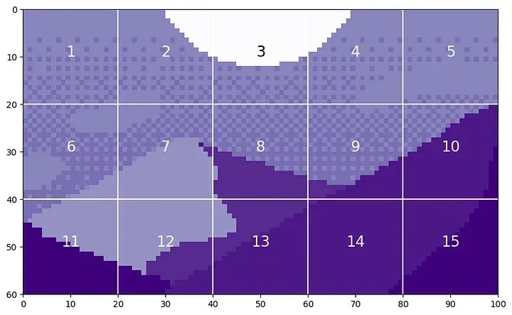
通过将这些补丁展平，我们可以看到生成的Token。让我们以第12个补丁为例，因为它包含了四种不同的色调。

print('Each patch will make a token of length', str(P**2)+'.')
print('\n')

patch12 = mountains[40:60, 20:40]
token12 = patch12.reshape(1, P**2)

fig = plt.figure(figsize=(10,1))
plt.imshow(token12, aspect=10, cmap='Purples_r')
plt.clim([0,1])
plt.xticks(np.arange(-0.5, 401, 50), labels=np.arange(0, 401, 50))
plt.yticks([]);
#plt.savefig(os.path.join(figure_path, 'mountain_token12.png'), bbox_inches='tight')

Each patch will make a token of length 400.

从图像中提取Token后，通常会使用线性投影来改变Token的长度。这通过一个可学习的线性层来实现。新的Token长度被称为潜在维度、通道维度或Token长度。在投影之后，Token不再能够在视觉上被识别为原始图像的补丁。现在我们理解了这个概念，我们可以看看补丁Token化是如何在代码中实现的。

class Patch_Tokenization(nn.Module):    
def __init__(self,         
       img_size: tuple[int, int, int]=(1, 1, 60, 100),                patch_size: int=50,           
       token_len: int=768):
       """ Patch Tokenization Module   
            Args:            
             img_size (tuple[int, int, int]): size of input (channels, height, width)           
              patch_size (int): the side length of a square patch                
              token_len (int): desired length of an output token        
              """    
              super().__init__()
              
              ## Defining Parameters  
              self.img_size = img_size    
              C, H, W = self.img_size     
              self.patch_size = patch_size   
              self.token_len = token_len    
              assert H % self.patch_size == 0, 'Height of image must be evenly divisible by patch size.'    
              assert W % self.patch_size == 0, 'Width of image must be evenly divisible by patch size.'    
              self.num_tokens = (H / self.patch_size) * (W / self.patch_size)
              
              ## Defining Layers    
              self.split = nn.Unfold(kernel_size=self.patch_size, stride=self.patch_size, padding=0)    
              self.project = nn.Linear((self.patch_size**2)*C, token_len)
   
              def forward(self, x): 
              x = self.split(x).transpose(1,0)    
              x = self.project(x)    
              return x

请注意两个断言语句，确保图像的尺寸可以被补丁大小整除。实际的补丁划分是通过一个torch.nn.Unfold⁵层实现的。

我们将使用我们裁剪的单通道版本的Mountain at Dusk⁴来运行此代码的示例。我们应该看到与之前相同的Token数量和初始Token大小的值。我们将使用token_len=768作为投影长度，这是基本变体的ViT²的大小。

下面代码块中的第一行是将Mountain at Dusk⁴的数据类型从NumPy数组更改为Torch张量。我们还必须对张量进行unsqueeze⁶操作，以创建一个通道维度和一个批处理大小维度。与上面一样，我们只有一个通道。由于只有一个图像，批处理大小为1。

x = torch.from_numpy(mountains).unsqueeze(0).unsqueeze(0).to(torch.float32)
token_len = 768
print('Input dimensions are\n\tbatchsize:', x.shape[0], '\n\tnumber of input channels:', x.shape[1], '\n\timage size:', (x.shape[2], x.shape[3]))

# Define the Module
patch_tokens = Patch_Tokenization(img_size=(x.shape[1], x.shape[2], x.shape[3]),                                   
                                    patch_size = P,      
                                    token_len = token_len)

Input dimensions are  
batchsize: 1  
number of input channels: 1   
image size: (60, 100)

正如我们在示例中看到的那样，共有N=15个长度为400的Token。最后，我们将Token投影为token_len。

x = patch_tokens.split(x).transpose(2,1)
print('After patch tokenization, dimensions are\n\tbatchsize:', x.shape[0], '\n\tnumber of tokens:', x.shape[1], '\n\ttoken length:', x.shape[2])

After patch tokenization, dimensions are  
  batchsize: 1   
  number of tokens: 15    
  token length: 400

现在我们有了Token，我们准备继续进行ViT。

Token Processing

我们将把ViT的下两个步骤，即编码块之前的步骤，称为“Token处理”。ViT图中的Token处理组件如下所示。

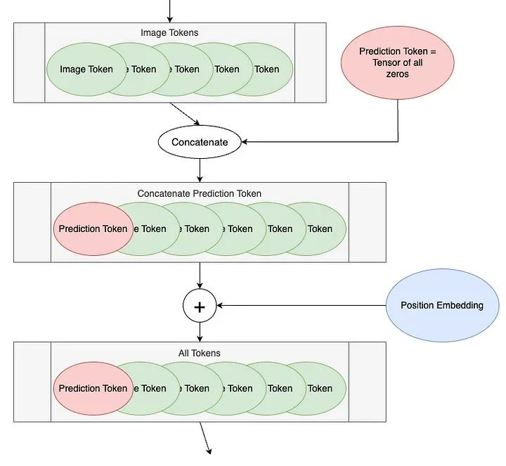
第一步是在图像Token之前添加一个空白Token，称为Prediction Token。此Token将用于输出编码块以进行预测。它最初是空白的 —— 等效于零 —— 这样它就可以从其他图像Token中获取信息。

# Define an Inpu
tnum_tokens = 175
token_len = 768
batch = 13
x = torch.rand(batch, num_tokens, token_len)
print('Input dimensions are\n\tbatchsize:', x.shape[0], '\n\tnumber of tokens:', x.shape[1], '\n\ttoken length:', x.shape[2])

# Append a Prediction Token
pred_token = torch.zeros(1, 1, token_len).expand(batch, -1, -1)
print('Prediction Token dimensions are\n\tbatchsize:', pred_token.shape[0], '\n\tnumber of tokens:', pred_token.shape[1], '\n\ttoken length:', pred_token.shape[2])

x = torch.cat((pred_token, x), dim=1)
print('Dimensions with Prediction Token are\n\tbatchsize:', x.shape[0], '\n\tnumber of tokens:', x.shape[1], '\n\ttoken length:', x.shape[2])

Input dimensions are  
    batchsize: 13   
    number of tokens: 175   
    token length: 768
Prediction Token dimensions are  
    batchsize: 13   
    number of tokens: 1   
    token length: 768
 Dimensions with Prediction Token are  
    batchsize: 13   
    number of tokens: 176    
    token length: 768

我们将从175个Token开始。每个Token的长度为768，这是ViT²基本变体的大小。我们使用批处理大小为13，因为它是素数，并且不会与任何其他参数混淆。

def get_sinusoid_encoding(num_tokens, token_len):   
   """ 
     Make Sinusoid Encoding Table

        Args:          
         num_tokens (int): number of tokens           
         token_len (int): length of a token
    Returns:           
     (torch.FloatTensor) sinusoidal position encoding table 
          
     """
     def get_position_angle_vec(i):       
     return [i / np.power(10000, 2 * (j // 2) / token_len) for j in range(token_len)]
     
     sinusoid_table = np.array([get_position_angle_vec(i) for i in range(num_tokens)])   
     sinusoid_table[:, 0::2] = np.sin(sinusoid_table[:, 0::2])   
     sinusoid_table[:, 1::2] = np.cos(sinusoid_table[:, 1::2]) 
    
    return torch.FloatTensor(sinusoid_table).unsqueeze(0)
    
PE = get_sinusoid_encoding(num_tokens+1, token_len)
print('Position embedding dimensions are\n\tnumber of tokens:', PE.shape[1], '\n\ttoken length:', PE.shape[2])

x = x + PE
print('Dimensions with Position Embedding are\n\tbatchsize:', x.shape[0], '\n\tnumber of tokens:', x.shape[1], '\n\ttoken length:', x.shape[2])

Position embedding dimensions are   number of tokens: 176    token length: 768Dimensions with Position Embedding are   batchsize: 13    number of tokens: 176    token length: 768

现在，我们为我们的Token添加了一个位置嵌入。位置嵌入允许Transformer理解图像token的顺序。请注意，这是一个增加，而不是一个连接。位置嵌入的具体细节是一个值得讨论的话题，最好留到以后再说。

def get_sinusoid_encoding(num_tokens, token_len):    """ Make Sinusoid Encoding Table
        Args:            num_tokens (int): number of tokens            token_len (int): length of a token
        Returns:            (torch.FloatTensor) sinusoidal position encoding table    """
    def get_position_angle_vec(i):        return [i / np.power(10000, 2 * (j // 2) / token_len) for j in range(token_len)]
    sinusoid_table = np.array([get_position_angle_vec(i) for i in range(num_tokens)])    sinusoid_table[:, 0::2] = np.sin(sinusoid_table[:, 0::2])    sinusoid_table[:, 1::2] = np.cos(sinusoid_table[:, 1::2]) 
    return torch.FloatTensor(sinusoid_table).unsqueeze(0)
PE = get_sinusoid_encoding(num_tokens+1, token_len)print('Position embedding dimensions are\n\tnumber of tokens:', PE.shape[1], '\n\ttoken length:', PE.shape[2])
x = x + PEprint('Dimensions with Position Embedding are\n\tbatchsize:', x.shape[0], '\n\tnumber of tokens:', x.shape[1], '\n\ttoken length:', x.shape[2])

Position embedding dimensions are   
  number of tokens: 176   
  token length: 768
Dimensions with Position Embedding are   
  batchsize: 13    
  number of tokens: 176    
  token length: 768

现在，我们的Token已经准备好进入编码块。

编码块

编码块是模型实际从图像标记中学习的地方。编码块的数量是用户设置的超参数。编码块的图表如下。

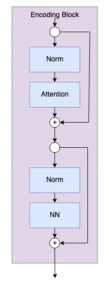
编码块的代码如下。

class Encoding(nn.Module):    def __init__(self,       dim: int,       num_heads: int=1,       hidden_chan_mul: float=4.,       qkv_bias: bool=False,       qk_scale: NoneFloat=None,       act_layer=nn.GELU,        norm_layer=nn.LayerNorm):                """ Encoding Block            Args:                dim (int): size of a single token                num_heads(int): number of attention heads in MSA                hidden_chan_mul (float): multiplier to determine the number of hidden channels (features) in the NeuralNet component                qkv_bias (bool): determines if the qkv layer learns an addative bias                qk_scale (NoneFloat): value to scale the queries and keys by;                                     if None, queries and keys are scaled by ``head_dim ** -0.5``                act_layer(nn.modules.activation): torch neural network layer class to use as activation                norm_layer(nn.modules.normalization): torch neural network layer class to use as normalization        """        super().__init__()        ## Define Layers        self.norm1 = norm_layer(dim)        self.attn = Attention(dim=dim,                            chan=dim,                            num_heads=num_heads,                            qkv_bias=qkv_bias,                            qk_scale=qk_scale)        self.norm2 = norm_layer(dim)        self.neuralnet = NeuralNet(in_chan=dim,                                hidden_chan=int(dim*hidden_chan_mul),                                out_chan=dim,                                act_layer=act_layer)    def forward(self, x):        x = x + self.attn(self.norm1(x))        x = x + self.neuralnet(self.norm2(x))        return x

num_heads 、qkv_bias和qk_scale参数定义了注意力模块组件。关于视觉转换器的注意力的深入研究留待下次再讨论。

hidden_ chan_mul和act_layer参数定义神经网络模块组件。激活层可以是任意⁷层。我们稍后torch.nn.modules.activation会详细介绍神经网络模块。

可以从任意⁸层中选择norm_layer torch.nn.modules.normalization。

现在，我们将逐步介绍图中的每个蓝色块及其附带的代码。我们将使用长度为 768 的 176 个标记。我们将使用批处理大小 13，因为它是素数，不会与任何其他参数混淆。我们将使用 4 个注意力头，因为它可以均匀划分标记长度；但是，您不会在编码块中看到注意力头维度。

# Define an Inputnum_tokens = 176token_len = 768batch = 13heads = 4x = torch.rand(batch, num_tokens, token_len)print('Input dimensions are\n\tbatchsize:', x.shape[0], '\n\tnumber of tokens:', x.shape[1], '\n\ttoken length:', x.shape[2])# Define the ModuleE = Encoding(dim=token_len, num_heads=heads, hidden_chan_mul=1.5, qkv_bias=False, qk_scale=None, act_layer=nn.GELU, norm_layer=nn.LayerNorm)E.eval();

Input dimensions are   batchsize: 13    number of tokens: 176    token length: 768

现在，我们将通过一个规范层和一个注意力模块。编码块中的注意力模块是参数化的，因此它不会改变标记长度。在注意力模块之后，我们实现了第一个拆分连接。

y = E.norm1(x)print('After norm, dimensions are\n\tbatchsize:', y.shape[0], '\n\tnumber of tokens:', y.shape[1], '\n\ttoken size:', y.shape[2])y = E.attn(y)print('After attention, dimensions are\n\tbatchsize:', y.shape[0], '\n\tnumber of tokens:', y.shape[1], '\n\ttoken size:', y.shape[2])y = y + xprint('After split connection, dimensions are\n\tbatchsize:', y.shape[0], '\n\tnumber of tokens:', y.shape[1], '\n\ttoken size:', y.shape[2])

After norm, dimensions are   batchsize: 13    number of tokens: 176    token size: 768After attention, dimensions are   batchsize: 13    number of tokens: 176    token size: 768After split connection, dimensions are   batchsize: 13    number of tokens: 176    token size: 768

现在，我们经过另一个规范层，然后是神经网络模块。最后是第二个拆分连接。

z = E.norm2(y)``
print('After norm, dimensions are\n\tbatchsize:', 
z.shape[0], '\n\tnumber of tokens:', z.shape[1], '\n\ttoken size:', z.shape[2])``z = E.neuralnet(z)``
print('After neural net, dimensions are\n\tbatchsize:',
 z.shape[0], '\n\tnumber of tokens:', z.shape[1], '\n\ttoken size:', z.shape[2])``
 z = z + y``
 print('After split connection, dimensions are\n\tbatchsize:', z.shape[0], '\n\tnumber of tokens:', z.shape[1], '\n\ttoken size:', z.shape[2])

After norm, dimensions are`  
  batchsize: 13   
  number of tokens: 176  
  token size: 768
After neural net, dimensions are
  batchsize: 13`   
  number of tokens: 176 
  token size: 768
After split connection, dimensions are
  batchsize: 13
  number of tokens: 176  
  token size: 768

这就是单个编码块的全部内容！由于最终维度与初始维度相同，模型可以轻松地通过多个编码块传递Token，由深度超参数设置。

神经网络模块

神经网络（NN）模块是编码块的子组件。NN模块非常简单，由一个全连接层、一个激活层和另一个全连接层组成。激活层可以是任何torch.nn.modules.activation⁷层，作为模块的输入传递。NN模块可以配置为改变输入的形状，或者保持相同的形状。我们不会逐步介绍这个代码，因为神经网络在机器学习中很常见，而且不是本文的重点。然而，下面给出了NN模块的代码。

class NeuralNet(nn.Module):
def __init__(self,
in_chan: int,
hidden_chan: NoneFloat=None,
out_chan: NoneFloat=None,
act_layer = nn.GELU):
""" Neural Network Module

Args:
in_chan (int): number of channels (features) at input
hidden_chan (NoneFloat): number of channels (features) in the hidden layer;
if None, number of channels in hidden layer is the same as the number of input channels
out_chan (NoneFloat): number of channels (features) at output;
if None, number of output channels is same as the number of input channels
act_layer(nn.modules.activation): torch neural network layer class to use as activation
"""

super().__init__()

## Define Number of Channels
hidden_chan = hidden_chan or in_chan

预测处理

通过编码块后，模型必须做的最后一件事是进行预测。ViT图中的“预测处理”组件如下所示。

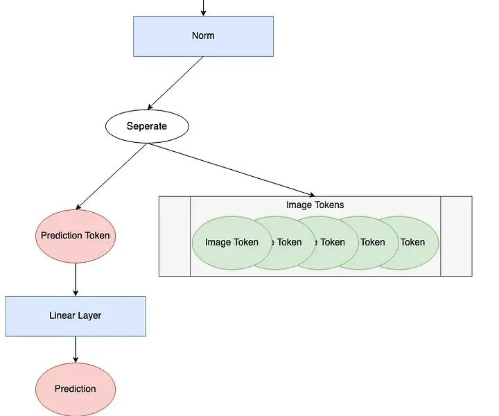
我们将查看该过程的每个步骤。我们将继续使用长度为768的176个Token。我们将使用批量大小为1来说明如何进行单个预测。批量大小大于1将会并行计算此预测。

在这里插入图片描述

首先，所有Token都通过一个norm层。

norm = nn.LayerNorm(token_len)
x = norm(x)
print('After norm, dimensions are\n\tbatchsize:', x.shape[0], '\n\tnumber of tokens:', x.shape[1], '\n\ttoken size:', x.shape[2])

接下来，我们从其余Token中分离出预测Token。在编码块中，预测Token已经变得非零，并获取了关于我们输入图像的信息。我们将仅使用此预测Token来进行最终预测。

在这里插入图片描述

最后，将预测Token传递到头部以进行预测。头部通常是某种类型的神经网络，根据模型的不同而变化。在An Image is Worth 16x16 Words²中，他们在预训练期间使用具有一个隐藏层的MLP（多层感知器），在微调期间使用单个线性层。在Tokens-to-Token ViT³中，他们使用单个线性层作为头部。此示例将使用输出形状为1，以表示单个估计回归值。

在这里插入图片描述

这就是全部内容！模型已经进行了预测！

完整代码

为了创建完整的ViT模块，我们使用上面定义的Patch Tokenization模块和ViT Backbone模块。ViT Backbone如下所定义，包含了Token处理、编码块和预测处理组件。


class ViT_Model(nn.Module): def __init__(self,    img_size: tuple[int, int, int]=(1, 400, 100),    patch_size: int=50,    token_len: int=768,    preds: int=1,    num_heads: int=1,    Encoding_hidden_chan_mul: float=4.,    depth: int=12,    qkv_bias=False,    qk_scale=None,    act_layer=nn.GELU,    norm_layer=nn.LayerNorm):
  """ VisTransformer Model
   Args:    img_size (tuple[int, int, int]): size of input (channels, height, width)    patch_size (int): the side length of a square patch    token_len (int): desired length of an output token    preds (int): number of predictions to output    num_heads(int): number of attention heads in MSA    Encoding_hidden_chan_mul (float): multiplier to determine the number of hidden channels (features) in the NeuralNet component of the Encoding Module    depth (int): number of encoding blocks in the model    qkv_bias (bool): determines if the qkv layer learns an addative bias    qk_scale (NoneFloat): value to scale the queries and keys by;          if None, queries and keys are scaled by ``head_dim ** -0.5``    act_layer(nn.modules.activation): torch neural network layer class to use as activation    norm_layer(nn.modules.normalization): torch neural network layer class to use as normalization  """  super().__init__()
  ## Defining Parameters  self.img_size = img_size  C, H, W = self.img_size  self.patch_size = patch_size  self.token_len = token_len  self.num_heads = num_heads  self.Encoding_hidden_chan_mul = Encoding_hidden_chan_mul  self.depth = depth
  ## Defining Patch Embedding Module  self.patch_tokens = Patch_Tokenization(img_size,           patch_size,           token_len)
  ## Defining ViT Backbone  self.backbone = ViT_Backbone(preds,         self.token_len,         self.num_heads,         self.Encoding_hidden_chan_mul,         self.depth,         qkv_bias,         qk_scale,         act_layer,         norm_layer)  ## Initialize the Weights  self.apply(self._init_weights)
 def _init_weights(self, m):  """ Initialize the weights of the linear layers & the layernorms  """  ## For Linear Layers  if isinstance(m, nn.Linear):   ## Weights are initialized from a truncated normal distrobution   timm.layers.trunc_normal_(m.weight, std=.02)   if isinstance(m, nn.Linear) and m.bias is not None:    ## If bias is present, bias is initialized at zero    nn.init.constant_(m.bias, 0)  ## For Layernorm Layers  elif isinstance(m, nn.LayerNorm):   ## Weights are initialized at one   nn.init.constant_(m.weight, 1.0)   ## Bias is initialized at zero   nn.init.constant_(m.bias, 0)
 @torch.jit.ignore ##Tell pytorch to not compile as TorchScript def no_weight_decay(self):  """ Used in Optimizer to ignore weight decay in the class token  """  return {'cls_token'}
 def forward(self, x):  x = self.patch_tokens(x)  x = self.backbone(x)  return x

通过ViT Backbone模块，我们可以定义完整的ViT模型。

   ``class ViT_Model(nn.Module):` `def __init__(self,`    `img_size: tuple[int, int, int]=(1, 400, 100),`    `patch_size: int=50,`    `token_len: int=768,`    `preds: int=1,`    `num_heads: int=1,`    `Encoding_hidden_chan_mul: float=4.,`    `depth: int=12,`    `qkv_bias=False,`    `qk_scale=None,`    `act_layer=nn.GELU,`    `norm_layer=nn.LayerNorm):``   `  `""" VisTransformer Model``   `   `Args:`    `img_size (tuple[int, int, int]): size of input (channels, height, width)`    `patch_size (int): the side length of a square patch`    `token_len (int): desired length of an output token`    `preds (int): number of predictions to output`    `num_heads(int): number of attention heads in MSA`    `Encoding_hidden_chan_mul (float): multiplier to determine the number of hidden channels (features) in the NeuralNet component of the Encoding Module`    `depth (int): number of encoding blocks in the model`    `qkv_bias (bool): determines if the qkv layer learns an addative bias`    `qk_scale (NoneFloat): value to scale the queries and keys by;``          if None, queries and keys are scaled by ``head_dim ** -0.5`` `    `act_layer(nn.modules.activation): torch neural network layer class to use as activation`    `norm_layer(nn.modules.normalization): torch neural network layer class to use as normalization`  `"""`  `super().__init__()``   `  `## Defining Parameters`  `self.img_size = img_size`  `C, H, W = self.img_size`  `self.patch_size = patch_size`  `self.token_len = token_len`  `self.num_heads = num_heads`  `self.Encoding_hidden_chan_mul = Encoding_hidden_chan_mul`  `self.depth = depth``   `  `## Defining Patch Embedding Module`  `self.patch_tokens = Patch_Tokenization(img_size,`           `patch_size,`           `token_len)``   `  `## Defining ViT Backbone`  `self.backbone = ViT_Backbone(preds,`         `self.token_len,`         `self.num_heads,`         `self.Encoding_hidden_chan_mul,`         `self.depth,`         `qkv_bias,`         `qk_scale,`         `act_layer,`         `norm_layer)`  `## Initialize the Weights`  `self.apply(self._init_weights)``   ` `def _init_weights(self, m):`  `""" Initialize the weights of the linear layers & the layernorms`  `"""`  `## For Linear Layers`  `if isinstance(m, nn.Linear):`   `## Weights are initialized from a truncated normal distrobution`   `timm.layers.trunc_normal_(m.weight, std=.02)`   `if isinstance(m, nn.Linear) and m.bias is not None:`    `## If bias is present, bias is initialized at zero`    `nn.init.constant_(m.bias, 0)`  `## For Layernorm Layers`  `elif isinstance(m, nn.LayerNorm):`   `## Weights are initialized at one`   `nn.init.constant_(m.weight, 1.0)`   `## Bias is initialized at zero`   `nn.init.constant_(m.bias, 0)``   ` `@torch.jit.ignore ##Tell pytorch to not compile as TorchScript` `def no_weight_decay(self):`  `""" Used in Optimizer to ignore weight decay in the class token`  `"""`  `return {'cls_token'}``   ` `def forward(self, x):`  `x = self.patch_tokens(x)`  `x = self.backbone(x)`  `return x

在ViT模型中，img_size、patch_size和token_len定义了Patch Tokenization模块。它们分别表示输入图像的大小、切分成的Patch的大小，以及由此生成的token序列的长度。正是通过这个模块，ViT将图像转化为模型能够处理的token序列。num_heads决定了多头注意力机制中“头”的数量；Encoding_hidden_channel_mul用于调整编码块的隐藏层通道数；qkv_bias和qk_scale则分别控制查询、键和值向量的偏置和缩放；而act_layer则代表激活函数层，我们可以选择任何torch.nn.modules.activation中的激活函数。此外，depth参数决定了模型中包含多少个这样的编码块。

norm_layer参数设置了编码块模块内外的norm。可以从任何torch.nn.modules.normalization⁸层中选择。

_init_weights方法来自于T2T-ViT³代码。此方法可以删除以随机初始化所有学习的权重和偏差。如实施的，线性层的权重被初始化为截断的正态分布；线性层的偏差被初始化为零；归一化层的权重被初始化为一；归一化层的偏差被初始化为零。

如何学习AI大模型？

大模型时代，火爆出圈的LLM大模型让程序员们开始重新评估自己的本领。 “AI会取代那些行业？”“谁的饭碗又将不保了？”等问题热议不断。

不如成为「掌握AI工具的技术人」，毕竟AI时代，谁先尝试，谁就能占得先机！

但是LLM相关的内容很多，现在网上的老课程老教材关于LLM又太少。所以现在小白入门就只能靠自学，学习成本和门槛很高

👉[CSDN大礼包🎁：全网最全《LLM大模型入门+进阶学习资源包》免费分享（安全链接，放心点击）]()👈

学习路线

在这里插入图片描述

第一阶段：从大模型系统设计入手，讲解大模型的主要方法；

第二阶段：在通过大模型提示词工程从Prompts角度入手更好发挥模型的作用；

第三阶段：大模型平台应用开发借助阿里云PAI平台构建电商领域虚拟试衣系统；

第四阶段：大模型知识库应用开发以LangChain框架为例，构建物流行业咨询智能问答系统；

第五阶段：大模型微调开发借助以大健康、新零售、新媒体领域构建适合当前领域大模型；

第六阶段：以SD多模态大模型为主，搭建了文生图小程序案例；

第七阶段：以大模型平台应用与开发为主，通过星火大模型，文心大模型等成熟大模型构建大模型行业应用。

在这里插入图片描述

👉学会后的收获：👈

• 基于大模型全栈工程实现（前端、后端、产品经理、设计、数据分析等），通过这门课可获得不同能力；

• 能够利用大模型解决相关实际项目需求：大数据时代，越来越多的企业和机构需要处理海量数据，利用大模型技术可以更好地处理这些数据，提高数据分析和决策的准确性。因此，掌握大模型应用开发技能，可以让程序员更好地应对实际项目需求；

• 基于大模型和企业数据AI应用开发，实现大模型理论、掌握GPU算力、硬件、LangChain开发框架和项目实战技能，学会Fine-tuning垂直训练大模型（数据准备、数据蒸馏、大模型部署）一站式掌握；

• 能够完成时下热门大模型垂直领域模型训练能力，提高程序员的编码能力：大模型应用开发需要掌握机器学习算法、深度学习框架等技术，这些技术的掌握可以提高程序员的编码能力和分析能力，让程序员更加熟练地编写高质量的代码。

在这里插入图片描述

1.AI大模型学习路线图
2.100套AI大模型商业化落地方案
3.100集大模型视频教程
4.200本大模型PDF书籍
5.LLM面试题合集
6.AI产品经理资源合集

👉获取方式：
😝有需要的小伙伴，可以保存图片到wx扫描二v码免费领取【保证100%免费】🆓

程序员丸子

关注

16
点赞
踩
17

收藏

觉得还不错? 一键收藏
0
评论
视觉Transformer解析(附代码)

自2017年**“注意力就是一切”**的理念问世以来，Transformer模型便迅速在自然语言处理（NLP）领域崭露头角，确立了其领先地位。到了2021年，“一张图片等于16x16个单词”的理念成功将Transformer模型引入计算机视觉任务中。自此之后，众多基于Transformer的架构纷纷涌现，应用于计算机视觉领域。本文将详细介绍“一张图片等于16x16个单词”中阐述的Vision Transformer（ViT），包括其开源代码和对各组件的概念解释。
复制链接

扫一扫