7/25 opencv-python学习笔记

.shap（)函数

img.shape[:2] 取彩色图片的长、宽。
如果img.shape[:3] 则取彩色图片的长、宽、通道。
关于img.shape[0]、[1]、[2]
img.shape[0]：图像的垂直尺寸（高度）
img.shape[1]：图像的水平尺寸（宽度）
img.shape[2]：图像的通道数
在矩阵中，[0]就表示行数，[1]则表示列数。

plt.subplot()

plt.subplot(nrows, ncols, index, **kwargs)
第一个参数：*args （官网文档描述）
Either a 3-digit integer or three separate integers describing the position of the subplot. If the three integers are nrows, ncols, and index in order, the subplot will take the index position on a grid with nrows rows and ncols columns. index starts at 1 in the upper left corner and increases to the right.
可以使用三个整数，或者三个独立的整数来描述子图的位置信息。如果三个整数是行数、列数和索引值，子图将分布在行列的索引位置上。索引从1开始，从右上角增加到右下角。
pos is a three digit integer, where the first digit is the number of rows, the second the number of columns, and the third the index of the subplot. i.e. fig.add_subplot(235) is the same as fig.add_subplot(2, 3, 5). Note that all integers must be less than 10 for this form to work.
位置是由三个整型数值构成，第一个代表行数，第二个代表列数，第三个代表索引位置。举个列子：plt.subplot(2, 3, 5) 和 plt.subplot(235) 是一样一样的。需要注意的是所有的数字不能超过10。

第二个参数：projection : {None, ‘aitoff’, ‘hammer’, ‘lambert’, ‘mollweide’, ‘polar’, ‘rectilinear’, str}, optional
The projection type of the subplot (Axes). str is the name of a costum projection, see projections. The default None results in a ‘rectilinear’ projection.
可选参数：可以选择子图的类型，比如选择polar，就是一个极点图。默认是none就是一个线形图。

第三个参数：polar : boolean, optional
If True, equivalent to projection=‘polar’. 如果选择true，就是一个极点图，上一个参数也能实现该功能。
官方文档传送门：plt.subplot()

plt.imshow()和plt.show()

plt.imshow(image) #image表示待处理的图像

plt.show()

原理：plt.imshow()函数负责对图像进行处理，并显示其格式，而plt.show()则是将plt.imshow()处理后的函数显示出来。

透视变换(persperctive transformation)

仿射变换都是在二维空间的变换，透视变换（投影变换）是在三维空间中发生了旋转。需要前后四组坐标来计算对应的转变矩阵，opencv提供了函数getPerspectiveTransform()来计算转变矩阵，cv2.wrapPerspective()函数来进行透视变换。其对应参数如下：

cv2.getPerspectiveTransform()   返回3*3的转变矩阵
        参数：    
            src：原图像中的四组坐标，如 np.float32([[56,65],[368,52],[28,387],[389,390]])
            dst: 转换后的对应四组坐标，如np.float32([[0,0],[300,0],[0,300],[300,300]])

            
        cv2.wrapPerspective()
        参数：    
            src: 图像对象
            M：3*3 transformation matrix (转变矩阵)
            dsize：输出矩阵的大小，注意格式为（cols，rows）  即width对应cols，height对应rows
            flags：可选，插值算法标识符，有默认值INTER_LINEAR，
                   如果插值算法为WARP_INVERSE_MAP, warpAffine函数使用如下矩阵进行图像转dst(x,y)=src(M11*x+M12*y+M13,M21*x+M22*y+M23)
            borderMode：可选， 边界像素模式，有默认值BORDER_CONSTANT 
            borderValue:可选，边界取值，有默认值Scalar()即0

官网使用示例：

img = cv2.imread('sudokusmall.png')
rows,cols,ch = img.shape

pts1 = np.float32([[56,65],[368,52],[28,387],[389,390]])
pts2 = np.float32([[0,0],[300,0],[0,300],[300,300]])

M = cv2.getPerspectiveTransform(pts1,pts2)

dst = cv2.warpPerspective(img,M,(300,300))

plt.subplot(121),plt.imshow(img),plt.title('Input')
plt.subplot(122),plt.imshow(dst),plt.title('Output')
plt.show()

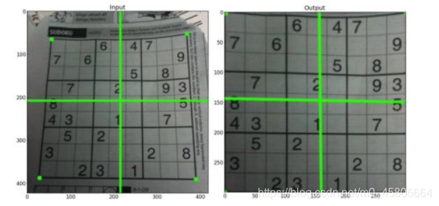
从上图中可以发现透视变换的一个应用，如果能找到原图中纸张的四个顶点，将其转换到新图中纸张的四个顶点，能将歪斜的roi区域转正，并进行放大；如在书籍，名片拍照上传后进行识别时，是一个很好的图片预处理方法。

对比度增强

对于部分图像，会出现整体较暗或较亮的情况，这是由于图片的灰度值范围较小，即对比度低。实际应用中，通过绘制图片的灰度直方图，可以很明显的判断图片的灰度值分布，区分其对比度高低。对于对比度较低的图片，可以通过一定的算法来增强其对比度。常用的方法有线性变换，伽马变换，直方图均衡化，局部自适应直方图均衡化等。

灰度直方图及绘制

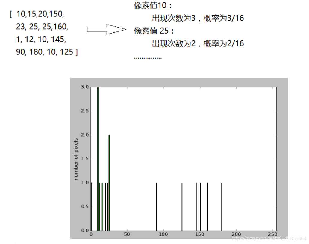
灰度直方图用来描述每个像素在图像矩阵中出现的次数或概率。其横坐标一般为0-255个像素值，纵坐标为该像素值对应的像素点个数。如下图所示的图像矩阵（单通道灰度图，三通道时可以分别绘制），可以统计每个像素值出现的次数，也可以统计概率，统计像素值出现次数的灰度直方图如下所示。

灰度直方图绘制
a, 可以利用opencv的calcHist()统计像素值出现次数，通过matploblib的plot()绘制
b, 可以直接利用matploblib的hist()方法

cv2.calcHist()
    参数：    
        img：输入图像，为列表，如[img]
        channels: 计算的通道，为列表，如[0]表示单通道,[0,1]统计两个通道
        mask: 掩模，和输入图像大小一样的矩阵，为1的地方会进行统计（与图像逻辑与后再统计）；无掩模时为None
        histSize: 每一个channel对应的bins个数，为列表，如[256]表示256个像素值
        ranges: bins的边界，为列表，如[0,256]表示像素值范围在0-256之间
        accumulate： Accumulation flag. If it is set, the histogram is not cleared in the beginning when it is allocated. This feature enables you to compute a single histogram from several sets of arrays, or to update the histogram in time.

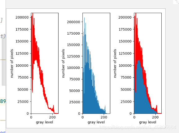
如下图所示，分别绘制了灰度分布曲线图，灰度分布直方图和两者叠加图形，代码如下：

import cv2 as cv
import matplotlib.pyplot as plt
import numpy as np
                
img = cv.imread(r"C:\Users\Administrator\Desktop\maze.png",0)

hist = cv.calcHist([img],[0],None,[256],[0,256])

plt.subplot(1,3,1),plt.plot(hist,color="r"),plt.axis([0,256,0,np.max(hist)])
plt.xlabel("gray level")
plt.ylabel("number of pixels")

plt.subplot(1,3,2),plt.hist(img.ravel(),bins=256,range=[0,256]),plt.xlim([0,256])
plt.xlabel("gray level")
plt.ylabel("number of pixels")

plt.subplot(1,3,3)
plt.plot(hist,color="r"),plt.axis([0,256,0,np.max(hist)])
plt.hist(img.ravel(),bins=256,range=[0,256]),plt.xlim([0,256])
plt.xlabel("gray level")
plt.ylabel("number of pixels")

plt.show()

原图

灰度直方图

c.通过np.histogram()和plt.hist()也可以计算出灰度值分布

import cv2 as cv
import matplotlib.pyplot as plt
import numpy as np


img = cv.imread(r"C:\Users\Administrator\Desktop\maze.png",0)
histogram,bins = np.histogram(img,bins=256,range=[0,256])
print(histogram)
plt.plot(histogram,color="g")
plt.axis([0,256,0,np.max(histogram)])
plt.xlabel("gray level")
plt.ylabel("number of pixels")
plt.show()

import cv2 as cv
import matplotlib.pyplot as plt
import numpy as np

img = cv.imread(r"C:\Users\Administrator\Desktop\maze.png",0)
rows,cols = img.shape
hist = img.reshape(rows*cols)
histogram,bins,patch = plt.hist(hist,256,facecolor="green",histtype="bar") #histogram即为统计出的灰度值分布
plt.xlabel("gray level")
plt.ylabel("number of pixels")
plt.axis([0,255,0,np.max(histogram)])
plt.show()

plt.hist()