【布线问题】“分支限界法”——《算法设计与分析（第五版）》

---

一、算法要求

印刷电路板将布线区域划分成m×n个方格阵列，精确的电路布线问题要求确定连接方格a的中点到方格b中点的最短布线方案。在布线时，电路只能沿直线或直角布线。

1. 思路

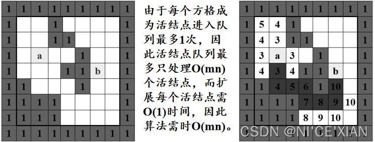
解此问题的队列式分支限界法从起始位置a（起始为2）开始将它作为第一个扩展结点。
与该扩展结点相邻并且可达的方格成为可行结点被加入到活结点队列中，并且将这些方格标记为3，即从起始方格a到这些方格的距离为3-2=1。
接着，算法从活结点队列中取出队首结点作为下一个扩展结点，并将与当前扩展结点相邻且未标记过的方格标记为4，并存入活结点队列。
这个过程一直继续到算法搜索到目标方格b或活结点队列为空时为止。即加入剪枝的广度优先搜索。

2. 示例

---

二、完整代码

1. 主文件

main.cpp：

//Project2: 布线问题

#include<iostream>
#include<iomanip>
#include<queue>
using namespace std;

const int length = 6;
int m = length,
    n = length,
    grid[length+2][length + 2];   

struct Position{
    int row, col;
};

void Print(){
    for (int i = 1; i < length+1; i++){
        for (int j = 1; j < length + 1; j++)
            cout << setw(3) << grid[i][j];
        cout << endl;
    }
    cout << endl;
}

bool FindPath(Position start, Position finish, int& PathLen, Position*& path){

    Position nextStep[4];
    nextStep[0].row = 0;nextStep[0].col = 1;//右
    nextStep[1].row = 1;nextStep[1].col = 0;//下
    nextStep[2].row = 0; nextStep[2].col = -1;//左
    nextStep[3].row = -1;nextStep[3].col = 0;//上

    Position here, next;
    here.row = start.row;
    here.col = start.col;
    grid[start.row][start.col] = 1;
    queue<Position> Q;

    while (true){ //标记相邻可达方格
        for (int i = 0; i < 4; i++){  //相邻四格 
            next.row = here.row + nextStep[i].row;
            next.col = here.col + nextStep[i].col;
            if (grid[next.row][next.col] == 0 && next.row != -1 && next.col != -1){ 
                grid[next.row][next.col] = grid[here.row][here.col] + 1; 		
                if ((next.row == finish.row) && (next.col == finish.col)) 
                    break; 

                Q.push(next);
            }
        }
        //截至条件
        if ((next.row == finish.row) && (next.col == finish.col)) 
            break;
        if (Q.empty()) return false;

        here = Q.front();
        Q.pop();

    }
    PathLen = grid[finish.row][finish.col];
    path = new Position[PathLen];
    //回溯
    here = finish;
    for (int j = PathLen - 1; j >= 0; j--){
        path[j] = here;
        //遍历四方向
        for (int i = 0; i < 4; i++){
            next.row = here.row + nextStep[i].row;
            next.col = here.col + nextStep[i].col;
            if (grid[next.row][next.col] == j){
                break;
            }
        }
        here = next;
    }
    return PathLen;
}
int main(){
    int countNum = 0;
    //阻碍
    grid[2][3] =  grid[3][4] = grid[3][5] = grid[4][2] = -1;

    Position start;//开始
    start.row = 2; start.col = 1;
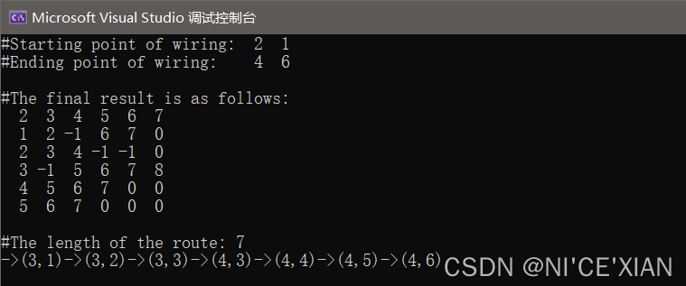
    cout << "#Starting point of wiring:"
        << setw(3) << start.row
        << setw(3) << start.col << endl;

    Position finish;//结束
    finish.row = 4;finish.col = 6;
    cout << "#Ending point of wiring:  "
        << setw(3) << finish.row
        << setw(3) << finish.col << endl;

    Position* path;
    FindPath(start, finish, countNum, path);
    cout << "\n#The final result is as follows: " << endl;
    Print();
    //最终结果
    cout << "#The length of the route: " << countNum - 1<< endl;
    for (int i = 1; i < countNum; i++){
        cout << "->(" << path[i].row
            << "," << path[i].col << ")";
    }
    cout << endl;

    return 0;
}

2. 效果展示

---

三、补充

算法复杂度分析:
(1）时间复杂度
分支限界法求布线问题，按照m叉树(m=4)的分析，空间树最坏情况下的结点为4ⁿ个，而空间树的深度n却是未知的，因此通过这种方法很难确定该算法的时间复杂度。那怎么办呢?我们要看看到底生成了多少个结点。
实际上，每个方格进入活结点队列最多1次，不会重复进入，因此对于m×n的方格阵列，活结点队列最多处理O(mn)个活结点，生成每个活结点需要O(1)的时间，因此算法时间复杂度为O(mn)。构造最短布线路径需要O(L)时间，其中L为最短布线路径长度。
(2）空间复杂度
空间复杂度为O(n)。

文档供本人学习笔记使用，仅供参考。