【深度学习21天学习挑战赛】2、复杂样本分类识别——卷积神经网络（CNN）服装图像分类

​

活动地址：CSDN21天学习挑战赛

完成了深度学习环境搭建和卷积神经网络（CNN）实现mnist手写数字识别的学习实践，最后总结了一下知识点，今天，继续跟着老师学习卷积神经网络（CNN）服装图像分类。

• 本文为🔗365天深度学习训练营 中的学习记录博客
• 参考文章地址： 🔗深度学习100例-卷积神经网络（CNN）服装图像分类 | 第3天
  

学习总结如下：（代码附后）

1、数据分析

1.1 了解fashion_mnist数据集

老师加载数据集： datasets.fashion_mnist.load_data()
用到的是：fashion_mnist数据集

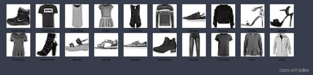
FashionMNIST 是一个图像数据集。 它是由一家德国的时尚科技公司提供。其涵盖了来自 10 种类别的共 7 万个不同商品的正面图片。FashionMNIST 的大小、格式和训练集/测试集划分与原始的 MNIST 完全一致。60000/10000的训练测试数据划分，28x28 的灰度图片。

数据分类说明：

标签值	分类
0	T恤 / 上衣 (T-shirt/top)
1	裤子 (Trouser)
2	套衫 (Pullover)
3	连衣裙 (Dress)
4	外套 (Coat)
5	凉鞋 (Sandal)
6	衬衫 (Shirt)
7	运动鞋 (Sneaker)
8	包 (Bag)
9	短靴 (Ankle boot)

数据可视化预览：

1.2 分析数据集

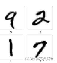
与刚刚学过的手写识别数据集相比较，这次的服装分类数据集特点明显，即像数据复杂度：服装分类的数据复杂度要明显高于手写数据。

数据大小：同样都是7 万个样本，训练集/测试集划分一致：60000/10000，28x28 的灰度图片。

分类情况：都是多分类（10分类）

2、模型搭建

与手写识别模型比较，多增加了一个卷积层，我们上节总结了，卷积层的作用是：用于从输入的高维数组中提取特征。卷积层的每个卷积核就是一个特征映射，用于提取某一个特征，卷积核的数量决定了卷积层输出特征个数 。

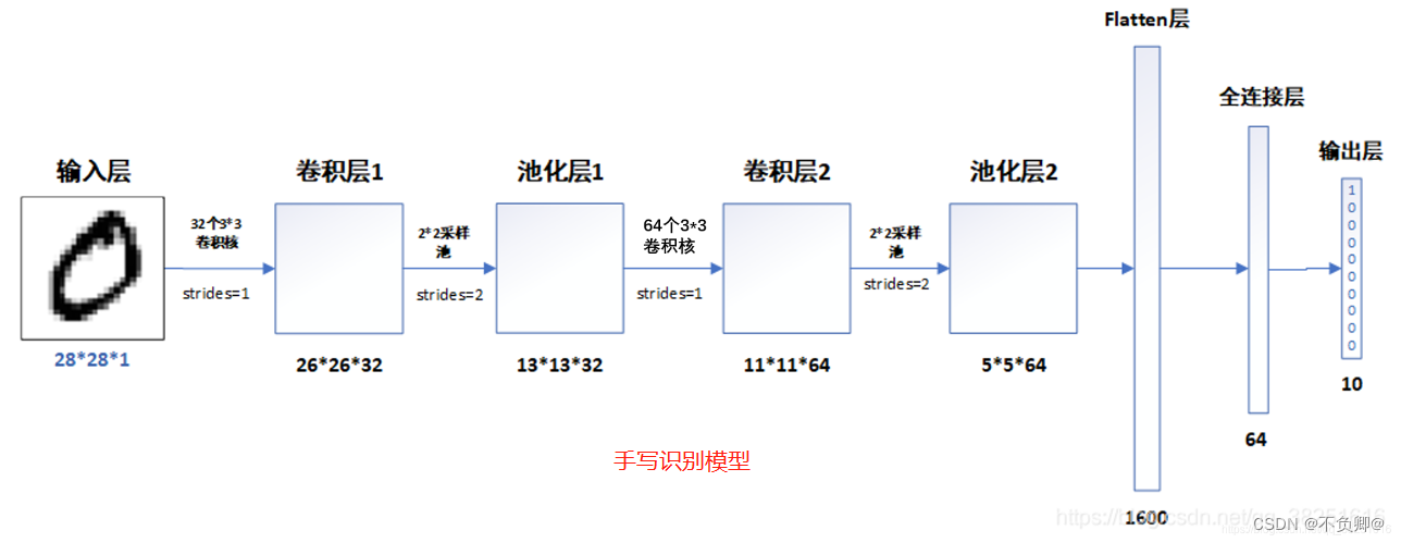
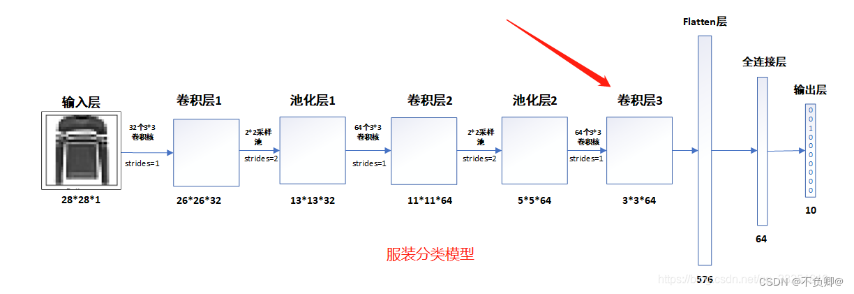
model = models.Sequential([
    layers.Conv2D(32, (3, 3), activation='relu', input_shape=(28, 28, 1)), #卷积层1，卷积核3*3
    layers.MaxPooling2D((2, 2)),                   #池化层1，2*2采样
    layers.Conv2D(64, (3, 3), activation='relu'),  #卷积层2，卷积核3*3
    layers.MaxPooling2D((2, 2)),                   #池化层2，2*2采样
    layers.Conv2D(64, (3, 3), activation='relu'),  #卷积层3，卷积核3*3
    
    layers.Flatten(),                      #Flatten层，连接卷积层与全连接层
    layers.Dense(64, activation='relu'),   #全连接层，特征进一步提取
    layers.Dense(10)                       #输出层，输出预期结果
])

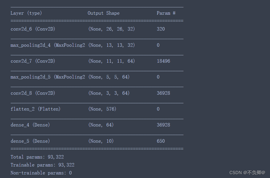
使用model.summary() ， 打印网络结构，如下：

3、配置模型

因为和手写识别模型一样，都是用于训练分类，所以，此处用到的优化器、损失函数、指标参数一致。

model.compile(optimizer='adam',
              loss=tf.keras.losses.SparseCategoricalCrossentropy(from_logits=True),
              metrics=['accuracy'])

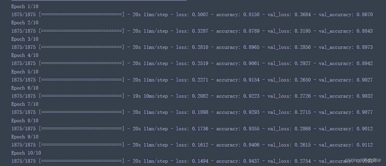
4、训练模型

history = model.fit(train_images, train_labels, epochs=10, 
                    validation_data=(test_images, test_labels))

• validation_data=(测试集输入特征，测试集标签)
• epochs = 迭代次数

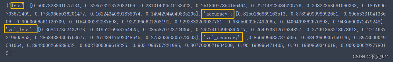
这里的history是接收模型训练返回的数据，其中包含：

• loss：训练集损失值
• accuracy：训练集准确率
• val_loss：测试集损失值
• val_accruacy：测试集准确率
  我们打印看看：print(history.history)
  

训练过程：

输出说明：

• loss：训练集损失值
• accuracy：训练集准确率
• val_loss：测试集损失值
• val_accruacy：测试集准确率

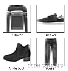
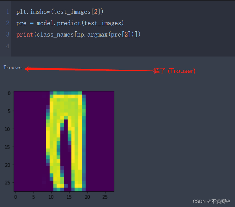
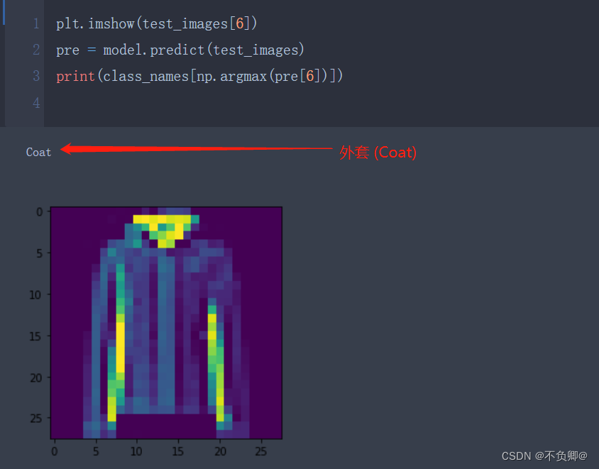
5、测试集预测

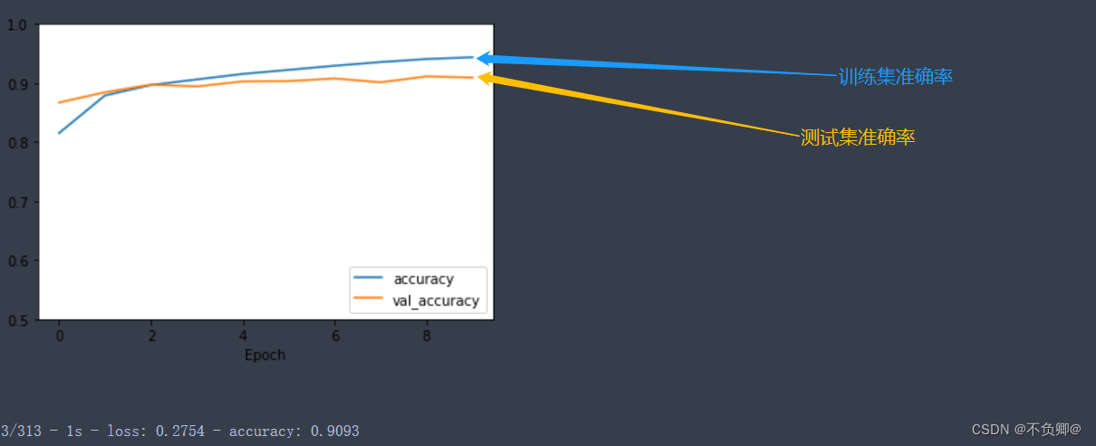
6、模型评估

plt.plot(history.history['accuracy'], label='accuracy')
plt.plot(history.history['val_accuracy'], label = 'val_accuracy')
plt.xlabel('Epoch')
plt.ylabel('Accuracy')
plt.ylim([0.5, 1])
plt.legend(loc='lower right')
plt.show()

test_loss, test_acc = model.evaluate(test_images,  test_labels, verbose=2)
print("测试准确率为：",test_acc)

7、完整代码

import tensorflow as tf
from tensorflow.keras import datasets, layers, models
import matplotlib.pyplot as plt
import numpy as np
(train_images, train_labels), (test_images, test_labels) = datasets.fashion_mnist.load_data() 
train_images, test_images = train_images / 255.0, test_images / 255.0 
#调整数据到我们需要的格式
train_images = train_images.reshape((60000, 28, 28, 1))
test_images = test_images.reshape((10000, 28, 28, 1))
class_names = ['T-shirt/top', 'Trouser', 'Pullover', 'Dress', 'Coat',
               'Sandal', 'Shirt', 'Sneaker', 'Bag', 'Ankle boot']
plt.figure(figsize=(20,10))
for i in range(20):
    plt.subplot(5,10,i+1)
    plt.xticks([])
    plt.yticks([])
    plt.grid(False)
    plt.imshow(train_images[i], cmap=plt.cm.binary)
    plt.xlabel(class_names[train_labels[i]])
plt.show()
model = models.Sequential([
    layers.Conv2D(32, (3, 3), activation='relu', input_shape=(28, 28, 1)), #卷积层1，卷积核3*3
    layers.MaxPooling2D((2, 2)),                   #池化层1，2*2采样
    layers.Conv2D(64, (3, 3), activation='relu'),  #卷积层2，卷积核3*3
    layers.MaxPooling2D((2, 2)),                   #池化层2，2*2采样
    layers.Conv2D(64, (3, 3), activation='relu'),  #卷积层3，卷积核3*3
    
    layers.Flatten(),                      #Flatten层，连接卷积层与全连接层
    layers.Dense(64, activation='relu'),   #全连接层，特征进一步提取
    layers.Dense(10)                       #输出层，输出预期结果
])
model.summary()
model.compile(optimizer='adam',
              loss=tf.keras.losses.SparseCategoricalCrossentropy(from_logits=True),
              metrics=['accuracy'])

history = model.fit(train_images, train_labels, epochs=10, 
                    validation_data=(test_images, test_labels))
plt.imshow(test_images[1])
pre = model.predict(test_images)
print(class_names[np.argmax(pre[1])])
plt.plot(history.history['accuracy'], label='accuracy')
plt.plot(history.history['val_accuracy'], label = 'val_accuracy')
plt.xlabel('Epoch')
plt.ylabel('Accuracy')
plt.ylim([0.5, 1])
plt.legend(loc='lower right')
plt.show()
test_loss, test_acc = model.evaluate(test_images,  test_labels, verbose=2)
print("测试准确率为：",test_acc)

学习日记

**
1，学习知识点

a、认识和使用fashion_mnist数据集
b、卷积神经网络（CNN）对复杂样本分类识别的基本使用
c、模型评估方法

2，学习遇到的问题

继续啃西瓜书，恶补基础