目标检测：RetinaNet算法细节以及代码部分

最新推荐文章于 2024-03-27 21:31:01 发布

追梦AI

最新推荐文章于 2024-03-27 21:31:01 发布

阅读量6.6k

点赞数

文章标签：深度学习 tensorflow 人工智能 pytorch 目标检测

本文链接：https://blog.csdn.net/m0_49100031/article/details/123349242

版权

一、背景

目标检测算法一般分为单阶段算法和多阶段算法。
多阶段算法特点是：精度高，但速度慢。（Faster-RCNN）
单阶段算法特点是：速度快，但精度不如前者。(SSD,RetinaNet，以及后面的FCOS等等)
精度低的关键原因就在于：正负样本极度不平衡。
那么Faster-RCNN为什么没有这个困扰？
因为在Faster-RCNN的RPN阶段已经对锚框进行了一个IOU匹配，做了一个筛选。
在SSD中，采用了难负样本挖掘来解决这个问题，但是还是有很多缺陷，主要有一下两个问题。
① 样本利用不充分：只使用了一小部分较难的负样本，大部分负样本都没有使用
② 挖掘难以控制：利用正样本数量的3倍来挖负样本，有时挖太多，有时挖太少
在RetinaNet通过修改标准交叉熵损失，提出了focal loss损失函数：
① 通过减少易分类样本的权重，使得模型在训练时更专注于难分类的样本，从而充分地利用所有样本
② 使得单阶段法检测器可以达到多阶段法检测器准确率，同时不影响原有的速度

二、算法细节

（1）RetinaNet对输入图像的操作：
① 随机水平翻转
② 单尺度训练：图像短边等比例缩放至800，且长边不超过1333
③ 多尺度训练：图像短边等比例缩放至[640, 672, 704, 736, 768, 800] ，
且长边不超过1333

class Augmenter(object):
    """以50%的概率进行随机翻转"""

    def __call__(self, sample, flip_x=0.5):

        if np.random.rand() < flip_x:
            image, annots = sample['img'], sample['annot']
            image = image[:, ::-1, :]

            rows, cols, channels = image.shape

            x1 = annots[:, 0].copy()
            x2 = annots[:, 2].copy()
            
            x_tmp = x1.copy()

            annots[:, 0] = cols - x2
            annots[:, 2] = cols - x_tmp

            sample = {'img': image, 'annot': annots}

        return sample

class Resizer(object):
    """Convert ndarrays in sample to Tensors."""
    # 论文中时min_side = 640,max_side=1333（单尺度训练时的参数）
    # 多尺度为至[640, 672, 704, 736, 768, 800] 且长边不超过1333
    def __call__(self, sample, min_side=608, max_side=1024):
        image, annots = sample['img'], sample['annot']
        rows, cols, cns = image.shape
        smallest_side = min(rows, cols)
        # 获取短边缩放比例
        scale = min_side / smallest_side
        largest_side = max(rows, cols)
        # 如果最大边大于max_side时，获得最大边缩放比例
        if largest_side * scale > max_side:
            scale = max_side / largest_side
        # 根据计算的比例调整图像的大小
        image = skimage.transform.resize(image, (int(round(rows*scale)), int(round((cols*scale)))))
        rows, cols, cns = image.shape
        # 为了保证长和宽是32的倍数，在周围填充了一圈，计算出需要填充的像素
        pad_w = 32 - rows%32
        pad_h = 32 - cols%32
        new_image = np.zeros((rows + pad_w, cols + pad_h, cns)).astype(np.float32)
        new_image[:rows, :cols, :] = image.astype(np.float32)
        # 取四位是box的信息，同样也需要乘以一定的比例去进行缩放
        annots[:, :4] *= scale

        return {'img': torch.from_numpy(new_image), 'annot': torch.from_numpy(annots), 'scale': scale}

（2）网络结构细节：
在这里插入图片描述 RetinaNet采用Resnet作为基础网络，ResNet有5个部分，Res1、 Res2、 Res3、 Res4、 Res5。
RetinaNet选取3个模块来作为初始的检测层 Res3、 Res4、 Res5。
如下图所示：
FPN过程：
Res5首先进行11卷积得到与上层相同通道数的特征图，再经过上采样的过程得到与上层大小相等的特征图，最后进行与上层特征图进行逐像素相加，最后在经过33卷积得到加强特征图。Res4，Res3操作时一样的。

# FPN
class PyramidFeatures(nn.Module):
    def __init__(self, C3_size, C4_size, C5_size, feature_size=256):
        super(PyramidFeatures, self).__init__()

        self.P5_1 = nn.Conv2d(C5_size, feature_size, kernel_size=1, stride=1, padding=0)
        self.P5_upsampled = nn.Upsample(scale_factor=2, mode='nearest')
        self.P5_2 = nn.Conv2d(feature_size, feature_size, kernel_size=3, stride=1, padding=1)

        self.P4_1 = nn.Conv2d(C4_size, feature_size, kernel_size=1, stride=1, padding=0)
        self.P4_upsampled = nn.Upsample(scale_factor=2, mode='nearest')
        self.P4_2 = nn.Conv2d(feature_size, feature_size, kernel_size=3, stride=1, padding=1)

        self.P3_1 = nn.Conv2d(C3_size, feature_size, kernel_size=1, stride=1, padding=0)
        self.P3_2 = nn.Conv2d(feature_size, feature_size, kernel_size=3, stride=1, padding=1)

        self.P6 = nn.Conv2d(C5_size, feature_size, kernel_size=3, stride=2, padding=1)

        self.P7_1 = nn.ReLU()
        self.P7_2 = nn.Conv2d(feature_size, feature_size, kernel_size=3, stride=2, padding=1)

    def forward(self, inputs):
        C3, C4, C5 = inputs

        P5_x = self.P5_1(C5)  # p5经过1*1卷积
        P5_upsampled_x = self.P5_upsampled(P5_x) # 上采样至与p4大小相等
        P5_x = self.P5_2(P5_x)  # 经过1*1卷积之后又经过3*3卷积得到最终的p5检测层

        P4_x = self.P4_1(C4) # p4经过1*1卷积
        P4_x = P5_upsampled_x + P4_x # p5上采样之后与p4逐像素相加
        P4_upsampled_x = self.P4_upsampled(P4_x) # p4上采样至与p3相等大小
        P4_x = self.P4_2(P4_x)  # p5上采样之后与p4逐像素相加再经过3*3卷积得到最终的p4检测层

        P3_x = self.P3_1(C3)  # p3经过1*1卷积
        P3_x = P3_x + P4_upsampled_x  # p4上采样之后与p3逐像素相加
        P3_x = self.P3_2(P3_x)  # p4上采样之后与p3逐像素相加再经过3*3卷积得到最终的p3检测层

        P6_x = self.P6(C5)  # C5检测层经过3*3卷积，stride=2 得到p6检测层

        P7_x = self.P7_1(P6_x)  # 经过relu激活函数
        P7_x = self.P7_2(P7_x)  # 经过3*3卷积，stride=2 得到p7检测层

        return [P3_x, P4_x, P5_x, P6_x, P7_x]

在这里插入图片描述
与FPN有差别的地方在于，RetinaNet还采用了P6,P7作为特征层与前三个基础检测层一起使用。
由上述代码得到P6,P7层是由P5进行stride=2的卷积操作得到，而不是下采样，P7是由P6经过RELU后在进行stride=2的卷积操作得到。这里引入P7层提升对大尺寸目标的检测效果。

（3） Anchors部分的细节：
• 从P3到P7层的anchors的面积从3232依次增加到512512。
• 每层anchors长宽比{1:2, 1:1, 2:1}，尺寸{2^0 , 2^1/3 , 2^2/3 } 与RPN比修改如下：
(1) anchor内部包含目标的判断仍然是与GT的IOU，IOU的阈值设置为0.5（RPN是 0.7）IOU大于0.5，anchors和GT关联；IOU在[0, 0.4)作为背景。
(2) 每个anchor最多关联一个GT。
(3) 边框回归就是计算anchor到关联的GT之间的偏移。

（4）分类子网络以及回归子网络

由上述图结构得知分类与回归都是一个4层卷积的网络，最后一层是用channel=KA(K是类别数，A是anchor数)的3×3卷积层，最后使用sigmoid激活函数。
为什么是KA？
Classification subnet 主要是用来预测每个位置上A个anchors属于K个类别的概率

class ClassificationModel(nn.Module):
    def __init__(self, num_features_in, num_anchors=9, num_classes=80, prior=0.01, feature_size=256):
        super(ClassificationModel, self).__init__()

        self.num_classes = num_classes
        self.num_anchors = num_anchors

        self.conv1 = nn.Conv2d(num_features_in, feature_size, kernel_size=3, padding=1)
        self.act1 = nn.ReLU()

        self.conv2 = nn.Conv2d(feature_size, feature_size, kernel_size=3, padding=1)
        self.act2 = nn.ReLU()

        self.conv3 = nn.Conv2d(feature_size, feature_size, kernel_size=3, padding=1)
        self.act3 = nn.ReLU()

        self.conv4 = nn.Conv2d(feature_size, feature_size, kernel_size=3, padding=1)
        self.act4 = nn.ReLU()

        self.output = nn.Conv2d(feature_size, num_anchors * num_classes, kernel_size=3, padding=1)
        self.output_act = nn.Sigmoid()

    def forward(self, x):
        out = self.conv1(x)
        out = self.act1(out)

        out = self.conv2(out)
        out = self.act2(out)

        out = self.conv3(out)
        out = self.act3(out)

        out = self.conv4(out)
        out = self.act4(out)

        out = self.output(out)
        out = self.output_act(out)

        # out is B x C x W x H, with C = n_classes + n_anchors
        out1 = out.permute(0, 2, 3, 1)

        batch_size, width, height, channels = out1.shape

        out2 = out1.view(batch_size, width, height, self.num_anchors, self.num_classes)

        return out2.contiguous().view(x.shape[0], -1, self.num_classes)

注意：这里分类子网络初始化除最后一层外都是采用σ = 0.01的高斯分布，偏置为0去做初始化。
最后一层偏置为− log((1 − π)/π)，π为每个anchor在开始训练时应该被标记为前景的置信度，实验中使用π = 0.01。背景远多于前景，所以 0.01的概率是前景。
原理：
一般流程：x经过
在这里插入图片描述
这样做的结果可以使得初始Loss更小。

回归子网络：

class RegressionModel(nn.Module):
    def __init__(self, num_features_in, num_anchors=9, feature_size=256):
        super(RegressionModel, self).__init__()

        self.conv1 = nn.Conv2d(num_features_in, feature_size, kernel_size=3, padding=1)
        self.act1 = nn.ReLU()

        self.conv2 = nn.Conv2d(feature_size, feature_size, kernel_size=3, padding=1)
        self.act2 = nn.ReLU()

        self.conv3 = nn.Conv2d(feature_size, feature_size, kernel_size=3, padding=1)
        self.act3 = nn.ReLU()

        self.conv4 = nn.Conv2d(feature_size, feature_size, kernel_size=3, padding=1)
        self.act4 = nn.ReLU()
        # num_anchors * 4 是一个anchors四个坐标
        self.output = nn.Conv2d(feature_size, num_anchors * 4, kernel_size=3, padding=1)
    # x为上述FPN某一层的feature map,经过4层卷积(ssd为1层)
    def forward(self, x):
        out = self.conv1(x)
        out = self.act1(out)

        out = self.conv2(out)
        out = self.act2(out)

        out = self.conv3(out)
        out = self.act3(out)

        out = self.conv4(out)
        out = self.act4(out)

        out = self.output(out)

        # out is B x C x W x H, with C = 4*num_anchors
        out = out.permute(0, 2, 3, 1)

        return out.contiguous().view(out.shape[0], -1, 4)

在最开始谈到的Focal Loss正是用于分类网络中，原理如下：
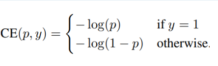
首先：二分类的交叉熵 (cross entropy, CE) 损失函数：
在这里插入图片描述
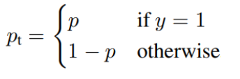
定义Pt为：

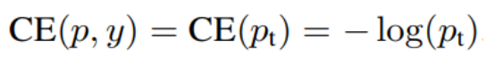
则可以简化为：

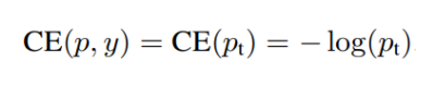
即：Pt 越接近于1，表示分类分的越正确
二分类的交叉熵 (cross entropy, CE) 损失函数：

Focal Loss为：

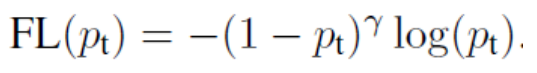
Pt 越接近于1，表示分类分的越正确
分类分的越正确，加权的权重越小

权重变化图如下：
在这里插入图片描述

追梦AI

关注

0
点赞
踩
15

收藏

觉得还不错? 一键收藏
0
评论
目标检测：RetinaNet算法细节以及代码部分

一、背景目标检测算法一般分为单阶段算法和多阶段算法。多阶段算法特点是：精度高，但速度慢。（Faster-RCNN）单阶段算法特点是：速度快，但精度不如前者。(SSD,RetinaNet，以及后面的FCOS等等)精度低的关键原因就在于：正负样本极度不平衡。那么Faster-RCNN为什么没有这个困扰？因为在Faster-RCNN的RPN阶段已经对锚框进行了一个IOU匹配，做了一个筛选。在SSD中，采用了难负样本挖掘来解决这个问题，但是还是有很多缺陷，主要有一下两个问题。① 样本利用不充分：只使
复制链接

扫一扫