NCL环流合成图的绘制（二）——NCL绘图基础

三.利用SST数据绘制环流合成图

1.SSTA composite

对于海表温度来说，我们通常研究其异常情况，因此本文首先读取已经处理过的海表温度异常值（SSTA）。

f = addfile("./ssta4d_flip.nc", "r")

我的目的是绘制某些特定年份中逐月SSTA的合成图,建立特定年份的index筛选并合成。合成分析一般t检验。

   ;composite
    nnumb_p = dimsizes (ind_piod2)

    sst_comp_p8 = dim_avg_n_Wrap(ssta(ind_piod2,8,:,:),0)
   ;t-test
    sst_std_p8 = dim_variance_n_Wrap(ssta(ind_piod2,8,:,:),0)
    sst_std_p8 = sqrt(sst_std_p8/nnumb_p)
    sst_std_p8 = where(sst_std_p8.eq.0,sst_std_p8@_FillValue,sst_std_p8)   
    t_sst_p8 = sst_comp_p8/sst_std_p8
    confi_sst_p8 = sst_comp_p8
    confi_sst_p8 = student_t(t_sst_p8, nnumb_p-1)
    printVarSummary(confi_sst_p8)

接下来设置绘图属性，在这里我才用全部填色然后对显著区域打点。

调用工作站并设置好图片分辨率

    wks_type = "png"
    wks_type@wkWidth = 2500
    wks_type@wkHeight = 2500 
    wks  = gsn_open_wks(wks_type,"composite_piod2")             

    base = new(1,graphic)

设置绘图属性并绘制

;;;;;res for composite
    res                      = True  
  
    res@gsnAddCyclic         = True
    res@gsnDraw              = False        ; don't draw yet
    res@gsnFrame             = False        ; don't advance frame yet
    res@gsnLeftString        = " "
    res@gsnRightString      = " "

    min_lon = min(ssta&longitude)
    max_lon = max(ssta&longitude)
    res@mpFillOn             = True
    res@mpCenterLonF         = 195.         ; defailt is 0 [GM]
    res@mpMinLatF            = -30.         ; zoom in on map
    res@mpMaxLatF            = 30.
    res@mpMinLonF            = min_lon
    res@mpMaxLonF            = max_lon

    res@pmTickMarkDisplayMode= "Always"
    res@mpGeophysicalLineThicknessF = 0.5
    res@mpGridAndLimbOn      = False
  
    res@cnFillOn             = True 
    res@cnLinesOn            = False                                
    res@cnLineLabelsOn       = False

    res@cnLevelSelectionMode = "ManualLevels"      ; manually set cn levels
    res@cnMinLevelValF       = -1.0                 ; min level
    res@cnMaxLevelValF       =  1.0                 ; max level
    res@cnLevelSpacingF      = .1                  ; contour level spacing
    res@cnFillPalette        = "cmp_b2r"   ; choose colormap
  
    res@mpPerimOn = True        
    res@cnInfoLabelOn        = False
    res@lbLabelBarOn        = False 
  
    res@lbLabelAutoStride = False
    res@cnLabelBarEndStyle   = "ExcludeOuterBoxes" 
    res@pmLabelBarWidthF     = 0.8

;;;;;plot composite 
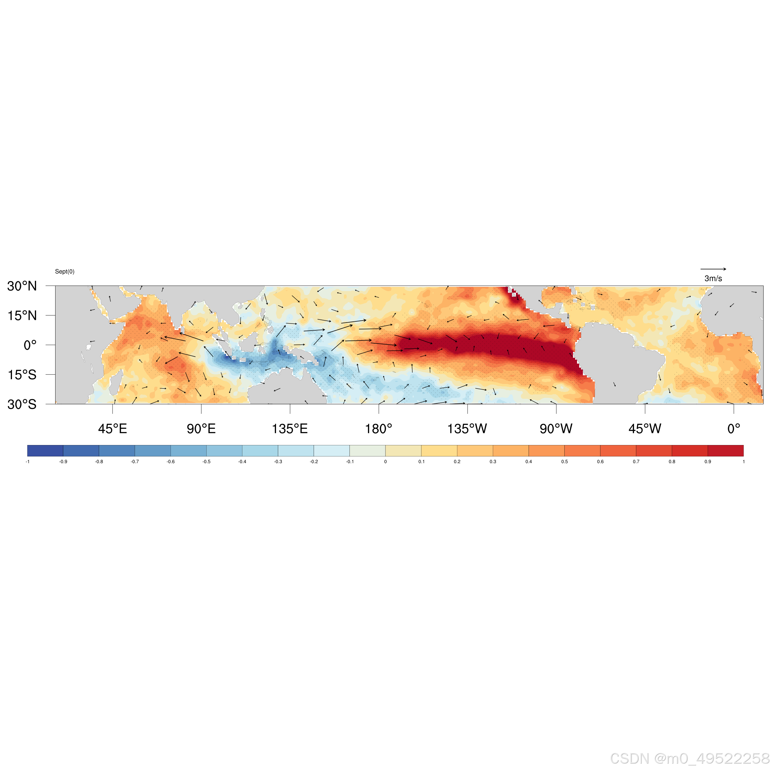
    res@gsnLeftString        = "Sept(0)"
    res@gsnLeftStringFontHeightF = 0.5
    base(0) = gsn_csm_contour_map(wks,sst_comp_p8,res) 

t-test

首先定义一个plot以便叠加。注意：只有底图才可以有地图_map，叠加图形中不可有地图，所以后面绘图函数不可调用gsn_csm_contour_map,而是gsn_csm_contour。

plot = new(1,graphic)

;;;;;t-test
    rest = True                            
    rest@gsnDraw             = False       
    rest@gsnFrame            = False 
    rest@gsnLeftString       = " "
    rest@gsnRightString      = " "      
    rest@cnInfoLabelOn       = False
    rest@cnLinesOn           = False       
    rest@cnLineLabelsOn      = False       
    rest@cnFillScaleF        = 0.5         
    rest@gsnAddCyclic        = True

    plot(0) = gsn_csm_contour(wks,confi_sst_p8,rest)
    
    opt = True
    opt@gsnShadeFillType = "pattern"
    opt@gsnShadeLow = 17
    opt@gsnAddCyclic         =True

    plot(0) = gsn_contour_shade(plot(0),  0.1, -999,  opt)
    overlay(base(0),plot(0))

2.风场绘制

首先读取UV分量

    f1 = addfile("./u4d.nc","r")
    f2 = addfile("./v4d.nc","r")
    u = f1->u4d
    printVarSummary(u)
    v = f2->v4d
    printVarSummary(v)

合成

    u_comp_p8 = dim_avg_n_Wrap(u(ind_piod2,8,:,:),0)
    v_comp_p8 = dim_avg_n_Wrap(v(ind_piod2,8,:,:),0)

检验

   ;u
    u_comp_p8 = dim_avg_n_Wrap(u(ind_piod2,8,:,:), 0)
    u_std_p8 = dim_variance_n_Wrap(u(ind_piod2,8,:,:), 0)
    u_std_p8 = sqrt(u_std_p8 / nnumb_p)
    u_std_p8 = where(u_std_p8.eq.0, u_std_p8@_FillValue, u_std_p8)
    t_u_p8 = u_comp_p8 / u_std_p8
    confi_u_p8 = student_t(t_u_p8, nnumb_p-1)
   ;v
    v_comp_p8 = dim_avg_n_Wrap(v(ind_piod2,8,:,:), 0)
    v_std_p8 = dim_variance_n_Wrap(v(ind_piod2,8,:,:), 0)
    v_std_p8 = sqrt(v_std_p8 / nnumb_p)
    v_std_p8 = where(v_std_p8.eq.0, v_std_p8@_FillValue, v_std_p8)
    t_v_p8 = v_comp_p8 / v_std_p8
    confi_v_p8 = student_t(t_v_p8, nnumb_p-1)

    u_comp_p8 = where(confi_u_p8.lt.0.1 .and. confi_v_p8.lt.0.1, 
u_comp_p8,u_comp_p8@_FillValue)
    v_comp_p8 = where(confi_u_p8.lt.0.1 .and. confi_v_p8.lt.0.1, v_comp_p8,v_comp_p8@_FillValue)

 

plotw = new(1,graphic) 

设置属性

;;;;;wind
    refmag = 3
    resw = True

    resw@gsnAddCyclic         = True        ; data not cyclic
    resw@gsnDraw              = False        ; don't draw yet
    resw@gsnFrame             = False        ; don't advance frame yet
    resw@gsnLeftString        = " "
    resw@gsnRightString      = " "

    resw@vcPositionMode = "ArrowTail"
    resw@vcGlyphStyle = "Fillarrow" 
    resw@vcFillArrowEdgeThicknessF = 2 
    resw@vcFillArrowEdgeColor = "black" 
    resw@vcFillArrowFillColor = "black"
    resw@vcFillArrowWidthF = 0.01 
    resw@vcFillArrowHeadXF = 0.1 
    resw@vcFillArrowHeadYF = 0.05 
    resw@vcFillArrowHeadInteriorXF = 0.05 
    resw@vcMinDistanceF = 0.02 
    resw@vcMinMagnitudeF = 0.5 

    resw@vcRefAnnoOn = True
    resw@vcRefMagnitudeF = refmag
    resw@vcRefLengthF = 0.03
    resw@vcRefAnnoBackgroundColor = "white"
    resw@vcRefAnnoPerimOn = False 
    resw@vcRefAnnoFontHeightF = 0.005
    resw@vcRefAnnoString1On = False
    resw@vcRefAnnoString2On = True
    resw@vcRefAnnoString2   = refmag + "m/s"
    resw@vcRefAnnoSide = "Top"
    resw@vcRefAnnoOrthogonalPosF = -0.12
    resw@vcRefAnnoParallelPosF = 0.95

    plotw(0) = gsn_csm_vector(wks, u_comp_p8,v_comp_p8, resw)
    overlay(base(0),plotw(0))

 这样我的环流合成图就完成啦