梯度检验（gradients checking）

3 - How does Gradient Checking work?
Backpropagation computes the gradients $\frac{\partial J}{\partial \theta }$, where $\theta$ denotes the parameters of the model. $J$ is computed using forward propagation and your loss function.

Because forward propagation is relatively easy to implement, you’re confident you got that right, and so you’re almost 100% sure that you’re computing the cost $J$ correctly. Thus, you can use your code for computing $J$ to verify the code for computing $\frac{\partial J}{\partial \theta }$.

Let’s look back at the definition of a derivative (or gradient):$$\frac{\partial J}{\partial \theta }=\underset{\epsilon \to 0}{\lim }\frac{J(\theta +\epsilon )-J(\theta -\epsilon )}{2\epsilon }$$

If you’re not familiar with the “$\underset{\epsilon \to 0}{\lim }$” notation, it’s just a way of saying “when $\epsilon$ is really, really small.”

You know the following:

$\frac{\partial J}{\partial \theta }$ is what you want to make sure you’re computing correctly.
You can compute $J(\theta +\epsilon )$ and $J(\theta -\epsilon )$ (in the case that $\theta$ is a real number), since you’re confident your implementation for $J$ is correct.
Let’s use equation (1) and a small value for $\epsilon$ to convince your CEO that your code for computing $\frac{\partial J}{\partial \theta }$ is correct!

• 主要方法就是将所有的参数压缩为一个很大的变量$\theta$，将神经网络看作为一个函数$F(\theta |Y)$,求参数的过程就是用微积分偏导数的定义
  $$grad=\underset{ϵ\to 0}{\lim }\frac{F(\theta +ϵ)-F(\theta -ϵ)}{2ϵ}$$
  使用上述公式对每一个参数进行检验。这非常消耗时间

# GRADED FUNCTION: gradient_check_n

def gradient_check_n(parameters, gradients, X, Y, epsilon=1e-7, print_msg=False):
    """
    Checks if backward_propagation_n computes correctly the gradient of the cost output by forward_propagation_n
    
    Arguments:
    parameters -- python dictionary containing your parameters "W1", "b1", "W2", "b2", "W3", "b3":
    grad -- output of backward_propagation_n, contains gradients of the cost with respect to the parameters. 
    x -- input datapoint, of shape (input size, 1)
    y -- true "label"
    epsilon -- tiny shift to the input to compute approximated gradient with formula(1)
    
    Returns:
    difference -- difference (2) between the approximated gradient and the backward propagation gradient
    """
    
    # Set-up variables
    parameters_values, _ = dictionary_to_vector(parameters)
    
    grad = gradients_to_vector(gradients)
    num_parameters = parameters_values.shape[0]
    J_plus = np.zeros((num_parameters, 1))
    J_minus = np.zeros((num_parameters, 1))
    gradapprox = np.zeros((num_parameters, 1))
    
    # Compute gradapprox
    for i in range(num_parameters):
        
        # Compute J_plus[i]. Inputs: "parameters_values, epsilon". Output = "J_plus[i]".
        # "_" is used because the function you have to outputs two parameters but we only care about the first one
        #(approx. 3 lines)
        # theta_plus =                                        # Step 1
        # theta_plus[i] =                                     # Step 2
        # J_plus[i], _ =                                     # Step 3
        # YOUR CODE STARTS HERE
        theta_plus = np.copy(parameters_values)
        theta_plus[i] = theta_plus[i] + epsilon
        J_plus[i],_ = forward_propagation_n(X,Y,vector_to_dictionary(theta_plus))
        # YOUR CODE ENDS HERE
        
        # Compute J_minus[i]. Inputs: "parameters_values, epsilon". Output = "J_minus[i]".
        #(approx. 3 lines)
        # theta_minus =                                    # Step 1
        # theta_minus[i] =                                 # Step 2        
        # J_minus[i], _ =                                 # Step 3
        # YOUR CODE STARTS HERE
        theta_minus = np.copy(parameters_values)
        theta_minus[i] = theta_minus[i]-epsilon
        J_minus[i],_ = forward_propagation_n(X,Y,vector_to_dictionary(theta_minus))
        # YOUR CODE ENDS HERE
        
        # Compute gradapprox[i]
        # (approx. 1 line)
        # gradapprox[i] = 
        # YOUR CODE STARTS HERE
        gradapprox[i] = (J_plus[i]-J_minus[i])/(2*epsilon)
        
        # YOUR CODE ENDS HERE
    
    # Compare gradapprox to backward propagation gradients by computing difference.
    # (approx. 1 line)
    # numerator =                                             # Step 1'
    # denominator =                                           # Step 2'
    # difference =                                            # Step 3'
    # YOUR CODE STARTS HERE
    numerator = np.linalg.norm(grad-gradapprox)
    denominator = np.linalg.norm(grad)+np.linalg.norm(gradapprox)
    difference = numerator/denominator
    print(vector_to_dictionary(grad-gradapprox))
    # YOUR CODE ENDS HERE
    if print_msg:
        if difference > 2e-7:
            print ("\033[93m" + "There is a mistake in the backward propagation! difference = " + str(difference) + "\033[0m")
        else:
            print ("\033[92m" + "Your backward propagation works perfectly fine! difference = " + str(difference) + "\033[0m")

    return difference

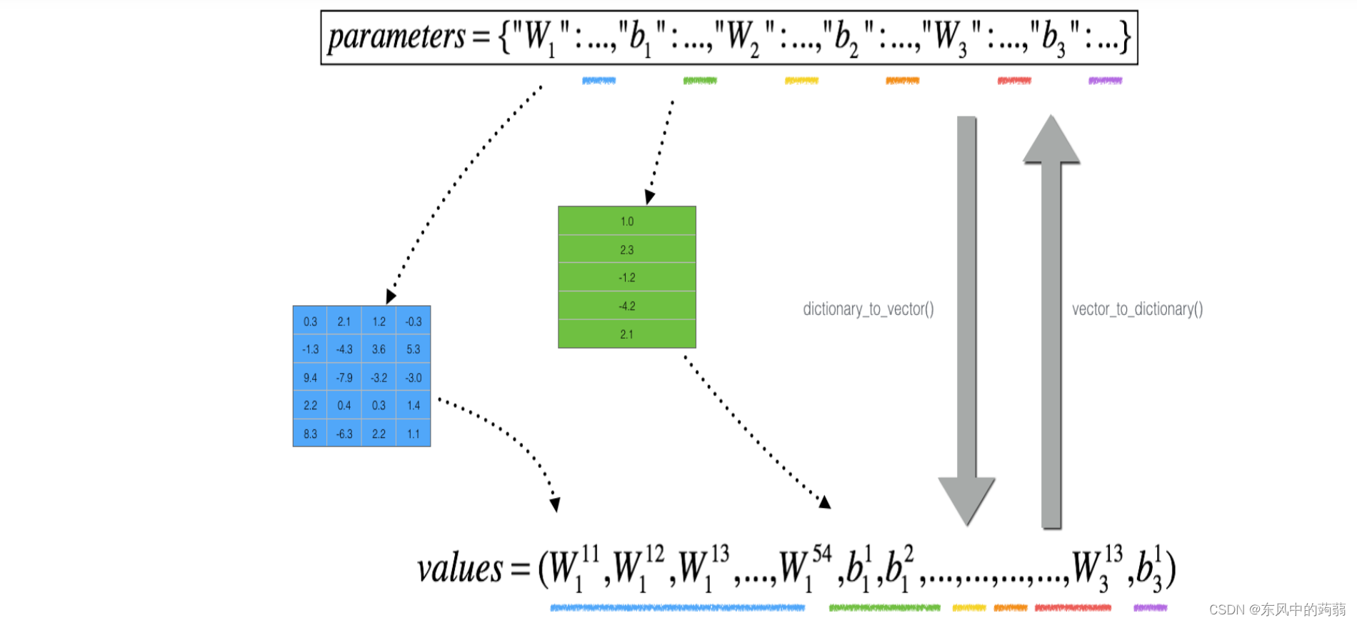
def dictionary_to_vector(parameters):
    """
    Roll all our parameters dictionary into a single vector satisfying our specific required shape.
    """
    keys = []
    count = 0
    for key in ["W1", "b1", "W2", "b2", "W3", "b3"]:
        
        # flatten parameter
        new_vector = np.reshape(parameters[key], (-1, 1))
        keys = keys + [key] * new_vector.shape[0]
        
        if count == 0:
            theta = new_vector
        else:
            theta = np.concatenate((theta, new_vector), axis=0)
        count = count + 1

    return theta, keys

def vector_to_dictionary(theta):
    """
    Unroll all our parameters dictionary from a single vector satisfying our specific required shape.
    """
    parameters = {}
    parameters["W1"] = theta[: 20].reshape((5, 4))
    parameters["b1"] = theta[20: 25].reshape((5, 1))
    parameters["W2"] = theta[25: 40].reshape((3, 5))
    parameters["b2"] = theta[40: 43].reshape((3, 1))
    parameters["W3"] = theta[43: 46].reshape((1, 3))
    parameters["b3"] = theta[46: 47].reshape((1, 1))

    return parameters

如果发现存在错误，可以将使用

vector_to_dictionary(grad-gradapprox)

将结果打印出来，从神经网络后面的参数往前观察，发现的第一个不为0的参数就是错误。

需要注意的是grad checking不能用于具有dropout正则化的网络，可以用于penalty的正则化。