


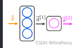
简单神经网络介绍
进入深度学习之前,先看看深度学习最重要的东西——神经网络
1.导入
import numpy as np
import matplotlib.pyplot as plt
plt.style.use('./deeplearning.mplstyle')
import tensorflow as tf
from tensorflow.keras.models import Sequential
from tensorflow.keras.layers import Dense
from lab_utils_common import dlc
from lab_coffee_utils import load_coffee_data, plt_roast, plt_prob, plt_layer, plt_network, plt_output_unit
import logging
logging.getLogger("tensorflow").setLevel(logging.ERROR)
tf.autograph.set_verbosity(0)
2.数据集导入及处理
2.1 导入数据集
X,Y = load_coffee_data();
print(X.shape, Y.shape)
这是关于烘焙咖啡的时间和温度烘焙出来的是否为好咖啡的数据集
2.2 数据可视化
plt_roast(X,Y)

2.3 归一化数据
如果数据归一化,将更快地对数据进行权重拟合(反向传播)。数据中的每个特征都被归一化为具有相似的范围。
下面的过程使用Keras normalization layer. 它有以下步骤:
- 创建“归一化层”(normalization layer)。注意,这不是模型中的层。
- “调整”数据。这将学习数据集的平均值和方差,并在内部保存这些值。
- 归一化数据。
将归一化应用于使用所学模型的任何未来数据非常重要。
3. Tensorflow 模型
3.1 模型建立
Sequential将各层线性排列,这里的3和1是units参数,指神经元数量,dense也是调的包
tf.random.set_seed(1234)  # applied to achieve consistent results 表示输入可为随机
model = Sequential(
    [
        tf.keras.Input(shape=(2,)),#表示输入是二维的
        Dense(3, activation='sigmoid', name = 'layer1'),
        Dense(1, activation='sigmoid', name = 'layer2') #提高数值稳定性
     ]
)
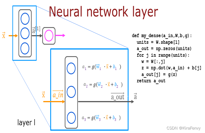
自己实现:
使用for循环访问层中的每个单元(j),并对该单元的权重(W[:,j])进行点积,然后求出单元(b[j])的偏差之和,形成z。然后可以将激活函数“g(z)”应用于该结果。
def my_dense(a_in, W, b, g):
    """
    Computes dense layer
    Args:
      a_in (ndarray (n, )) : Data, 1 example
      W    (ndarray (n,j)) : Weight matrix, n features per unit, j units
      b    (ndarray (j, )) : bias vector, j units
      g    activation function (e.g. sigmoid, relu..)
    Returns
      a_out (ndarray (j,))  : j units|
    """
    units = W.shape[1]
    a_out = np.zeros(units)
    for j in range(units):
        w = W[:,j]
        z = np.dot(w, a_in) + b[j]
        a_out[j] = g(z)
    return(a_out)

def my_sequential(x, W1, b1, W2, b2):
    a1 = my_dense(x,  W1, b1, sigmoid)
    a2 = my_dense(a1, W2, b2, sigmoid)
    return(a2)
sigmoid函数其实不适合在最后一层出现,会导致稳定性增加
3.2 检查
看看模型情况
model.summary()

Model: "sequential"
_________________________________________________________________
 Layer (type)                Output Shape              Param #
=================================================================
 layer1 (Dense)              (None, 3)                 9

 layer2 (Dense)              (None, 1)                 4

=================================================================
Total params: 13
Trainable params: 13
Non-trainable params: 0
_________________________________________________________________
这是参数数量,第一个隐藏层有3个神经元,每个神经元2个w参数1个b参数,第二个隐藏层有1个神经元,含3个w参数1个b参数
L1_num_params = 2 * 3 + 3   # W1 parameters  + b1 parameters
L2_num_params = 3 * 1 + 1   # W2 parameters  + b2 parameters
print("L1 params = ", L1_num_params, ", L2 params = ", L2_num_params  )
可以检查一下
W1, b1 = model.get_layer("layer1").get_weights()
W2, b2 = model.get_layer("layer2").get_weights()
print(f"W1{W1.shape}:\n", W1, f"\nb1{b1.shape}:", b1)
print(f"W2{W2.shape}:\n", W2, f"\nb2{b2.shape}:", b2)


W1(2, 3):
 [[-0.8  -0.85  1.03]
 [-0.05 -0.16 -0.17]]
b1(3,): [0. 0. 0.]
W2(3, 1):
 [[-0.37]
 [ 0.65]
 [ 0.58]]
b2(1,): [0.]
3.3 模型运行
- The
model.compilestatement defines a loss function and specifies a compile optimization. 定义了一个损失函数,指定了一个编译优化器 - The
model.fitstatement runs gradient descent and fits the weights to the data. 运行梯度下降,把权重拟合到数据
model.compile(
    loss = tf.keras.losses.BinaryCrossentropy(),
    optimizer = tf.keras.optimizers.Adam(learning_rate=0.01),
)

model.fit(
    Xt,Yt,
    epochs=10,
)

Epoch 1/10
6250/6250 [==============================] - 9s 1ms/step - loss: 0.1855
Epoch 2/10
6250/6250 [==============================] - 8s 1ms/step - loss: 0.1168
……
Epoch 10/10
6250/6250 [==============================] - 9s 1ms/step - loss: 0.0017
查看更新过的weight
W1, b1 = model.get_layer("layer1").get_weights()
W2, b2 = model.get_layer("layer2").get_weights()
print("W1:\n", W1, "\nb1:", b1)
print("W2:\n", W2, "\nb2:", b2)

W1:
 [[ 14.62   0.18 -11.11]
 [ 12.12  10.38  -0.31]]
b1: [  2.    12.52 -11.95]
W2:
 [[-46.16]
 [ 44.21]
 [-53.99]]
b2: [-13.75]
3.4 预测
调用predict函数
X_test = np.array([
    [200,13.9],  # postive example
    [200,17]])   # negative example
X_testn = norm_l(X_test)
predictions = model.predict(X_testn)
print("predictions = \n", predictions)

1/1 [==============================] - 0s 81ms/step
predictions =
 [[9.93e-01]
 [1.49e-07]]
当然也可以手写predict函数
def my_predict(X, W1, b1, W2, b2):
    m = X.shape[0]
    p = np.zeros((m,1))
    for i in range(m):
        p[i,0] = my_sequential(X[i], W1, b1, W2, b2)
    return(p)
Epochs and batches
- “epochs”的数量被设置为10。这指定整个数据集应在训练期间应用10次(10个循环或10次迭代)
- batch的默认值为32,
6250/6250[====描述了已执行的batch(批处理)
3.5 转换为决策
To convert the probabilities to a decision, we apply a threshold: 将概率转化为决策
yhat = np.zeros_like(predictions)#初始化一个与predictions相同形状和类型的数组来存储决策结果
for i in range(len(predictions)):
    if predictions[i] >= 0.5:
        yhat[i] = 1
    else:
        yhat[i] = 0
print(f"decisions = \n{yhat}")

decisions =
[[1.]
 [0.]]
简洁版
yhat = (predictions >= 0.5).astype(int) #astype
print(f"decisions = \n{yhat}")

decisions =
[[1]
 [0]]
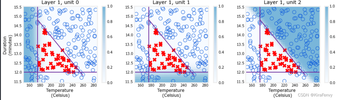
3.6 可视化
可视化第一层
def plt_layer(X,Y,W1,b1,norm_l): # 可以学学如何画图
    Y = Y.reshape(-1,)
    fig,ax = plt.subplots(1,W1.shape[1], figsize=(16,4))
    for i in range(W1.shape[1]):
        layerf= lambda x : sigmoid(np.dot(norm_l(x),W1[:,i]) + b1[i])
        plt_prob(ax[i], layerf)
        ax[i].scatter(X[Y==1,0],X[Y==1,1], s=70, marker='x', c='red', label="Good Roast" )
        ax[i].scatter(X[Y==0,0],X[Y==0,1], s=100, marker='o', facecolors='none',
                   edgecolors=dlc["dldarkblue"],linewidth=1,  label="Bad Roast")
        tr = np.linspace(175,260,50)
        ax[i].plot(tr, (-3/85) * tr + 21, color=dlc["dlpurple"],linewidth=2)
        ax[i].axhline(y= 12, color=dlc["dlpurple"], linewidth=2)
        ax[i].axvline(x=175, color=dlc["dlpurple"], linewidth=2)
        ax[i].set_title(f"Layer 1, unit {i}")
        ax[i].set_xlabel("Temperature \n(Celsius)",size=12)
    ax[0].set_ylabel("Duration \n(minutes)",size=12)
    plt.show()

plt_layer(X,Y.reshape(-1,),W1,b1,norm_l)
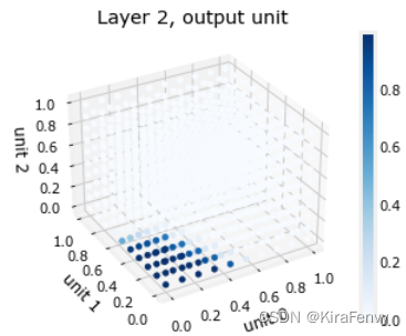
可视化第二层输出:
它的输入是第一层的输出。我们知道第一层使用的是sigmoid,因此它们的输出范围在0到1之间。我们可以创建一个三维绘图,计算三个输入的所有可能组合的输出。
plt_output_unit(W2,b2)
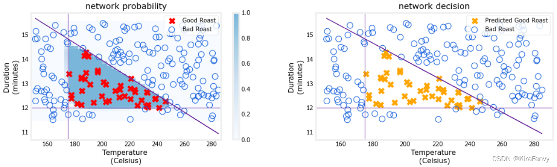
3.7 绘制网络
def plt_network(X,Y,netf):
    fig, ax = plt.subplots(1,2,figsize=(16,4))
    Y = Y.reshape(-1,)
    plt_prob(ax[0], netf)
    ax[0].scatter(X[Y==1,0],X[Y==1,1], s=70, marker='x', c='red', label="Good Roast" )
    ax[0].scatter(X[Y==0,0],X[Y==0,1], s=100, marker='o', facecolors='none',
                   edgecolors=dlc["dldarkblue"],linewidth=1,  label="Bad Roast")
    ax[0].plot(X[:,0], (-3/85) * X[:,0] + 21, color=dlc["dlpurple"],linewidth=1)
    ax[0].axhline(y= 12, color=dlc["dlpurple"], linewidth=1)
    ax[0].axvline(x=175, color=dlc["dlpurple"], linewidth=1)
    ax[0].set_xlabel("Temperature \n(Celsius)",size=12)
    ax[0].set_ylabel("Duration \n(minutes)",size=12)
    ax[0].legend(loc='upper right')
    ax[0].set_title(f"network probability")

    ax[1].plot(X[:,0], (-3/85) * X[:,0] + 21, color=dlc["dlpurple"],linewidth=1)
    ax[1].axhline(y= 12, color=dlc["dlpurple"], linewidth=1)
    ax[1].axvline(x=175, color=dlc["dlpurple"], linewidth=1)
    fwb = netf(X)
    yhat = (fwb > 0.5).astype(int)
    ax[1].scatter(X[yhat[:,0]==1,0],X[yhat[:,0]==1,1], s=70, marker='x', c='orange', label="Predicted Good Roast" )
    ax[1].scatter(X[yhat[:,0]==0,0],X[yhat[:,0]==0,1], s=100, marker='o', facecolors='none',
                   edgecolors=dlc["dldarkblue"],linewidth=1,  label="Bad Roast")
    ax[1].set_title(f"network decision")
    ax[1].set_xlabel("Temperature \n(Celsius)",size=12)
    ax[1].set_ylabel("Duration \n(minutes)",size=12)
    ax[1].legend(loc='upper right')
netf= lambda x : model.pr

edict(norm_l(x))
plt_network(X,Y,netf)
4.课后题
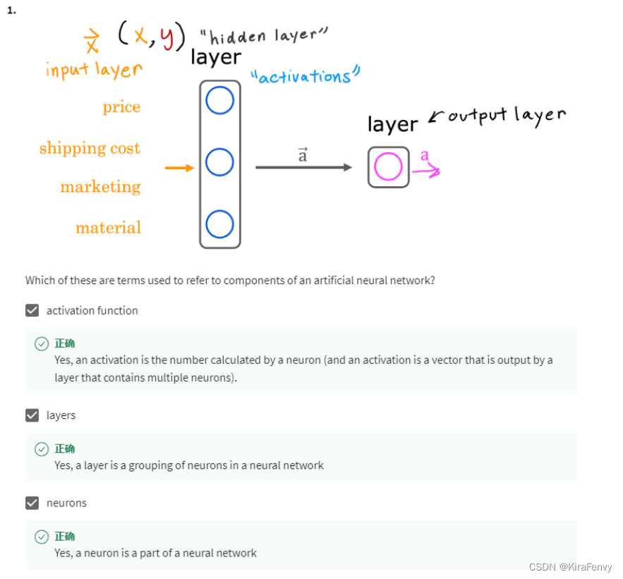
- 激活函数是神经元当中计算的东西,输入经过激活函数得到输出,一个layer由一组神经元组成
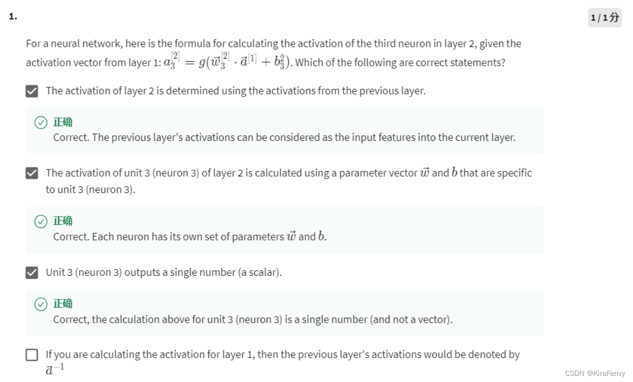
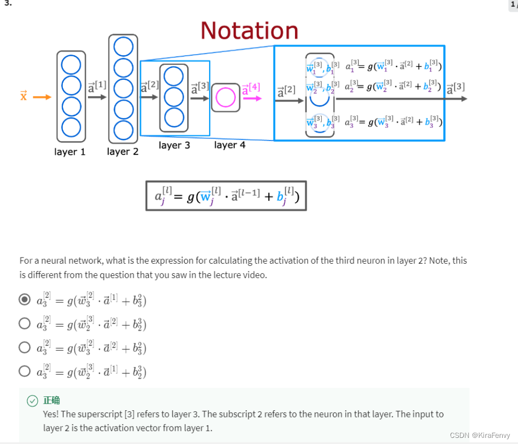
- 这里的 w [ 2 ] w^{[2]} w[2]代表是第二层的w, a [ 1 ] a^{[1]} a[1]代表第一层输出的a,下标的3表示第3个神经元
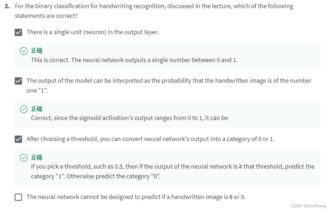
- 二分类问题,只输出一个值范围在0-1
4. 公式表述相关,注意上下标,上标含义为层数,下标含义为神经元数
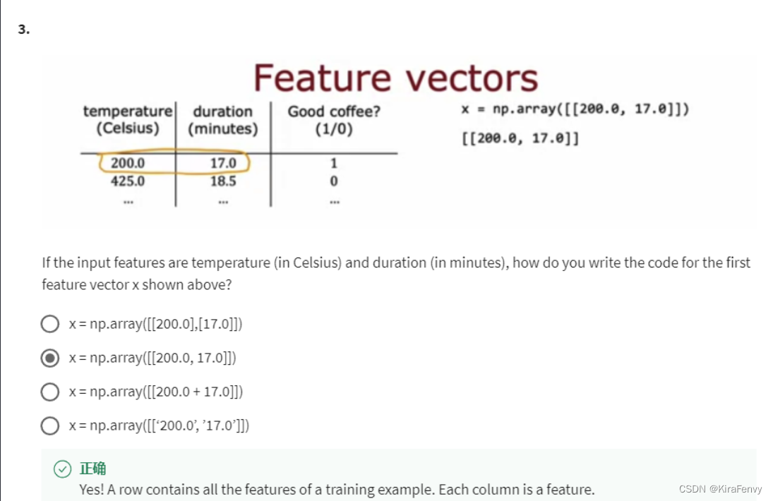
5. 一般一个数据按行,一个特征按列
6. 前向传播的实现
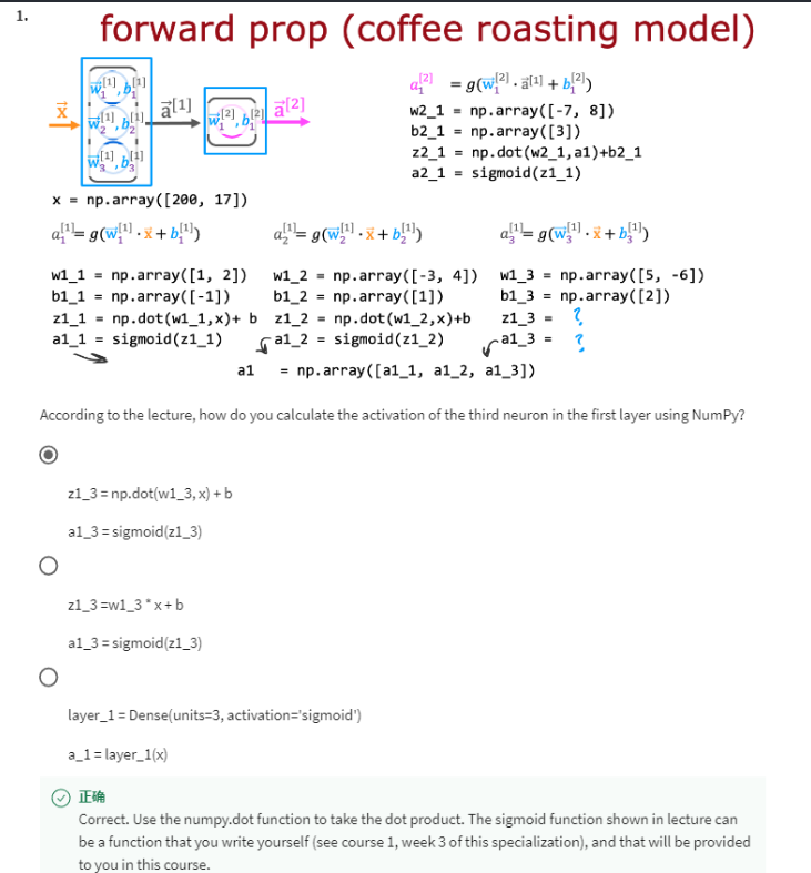
7. 注意,同一行证明都是同一项w,同一列证明同一个神经元
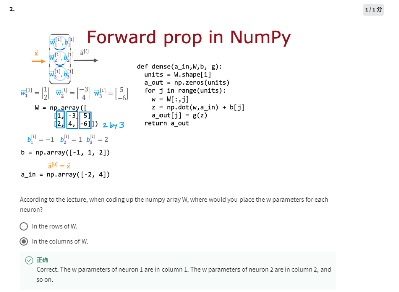
8. 对于定义单个神经元层的“dense”函数中的上述代码,该代码需要多少次
“for循环”?请注意,W有2行3列。
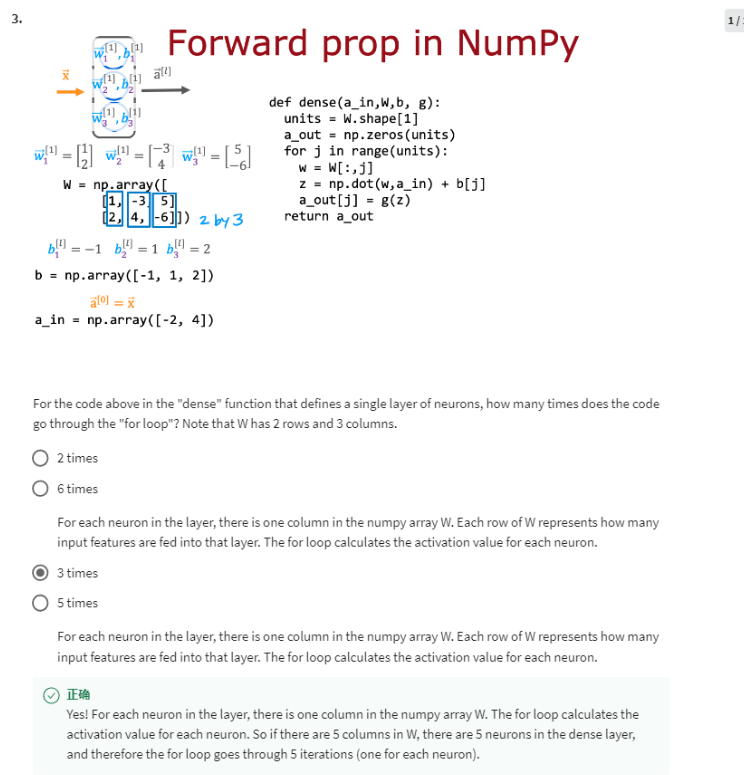
对于层中的每个神经元,numpy数组W中有一列。每行W代表多少输入特征被输入到该层中。for循环计算每个神经元的激活值,有3列就是3个神经元,就是3次循环。


 1984
1984


 被折叠的 条评论
为什么被折叠?
被折叠的 条评论
为什么被折叠?
 到【灌水乐园】发言


