【Machine Learning】16.激活函数ReLU

之前激活函数几乎就只用sigmoid，然而实际上有很多激活函数可以用，本文介绍ReLU函数的使用

ReLU全拼Rectified Linear Unit，直译矫正过的线性单元，不过意思相当于保留数据的正数部分，负数部分全部变为0

1.导入

注意layers和activations的导入

import numpy as np
import matplotlib.pyplot as plt
from matplotlib.gridspec import GridSpec
plt.style.use('./deeplearning.mplstyle')
import tensorflow as tf
from tensorflow.keras.models import Sequential
from tensorflow.keras.layers import Dense, LeakyReLU
from tensorflow.keras.activations import linear, relu, sigmoid
%matplotlib inline
from matplotlib.widgets import Slider
from lab_utils_common import dlc
from autils import plt_act_trio
from lab_utils_relu import *
import warnings
warnings.simplefilter(action='ignore', category=UserWarning)

2.ReLU介绍

激活函数
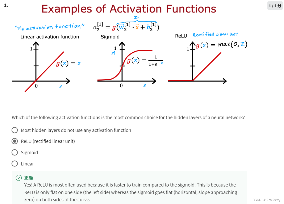
这里有三种不同的激活函数

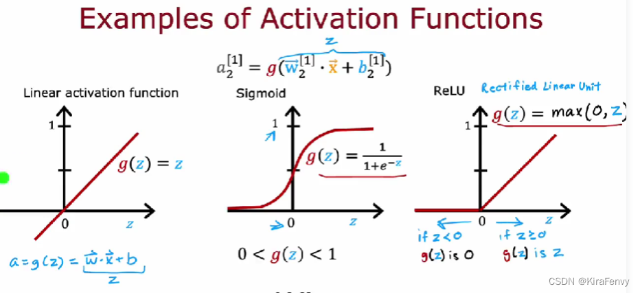
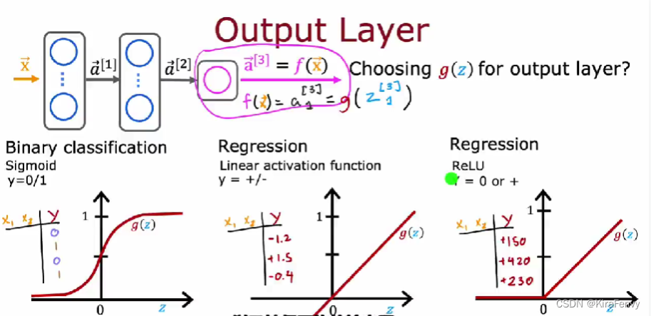
如何选择激活函数？

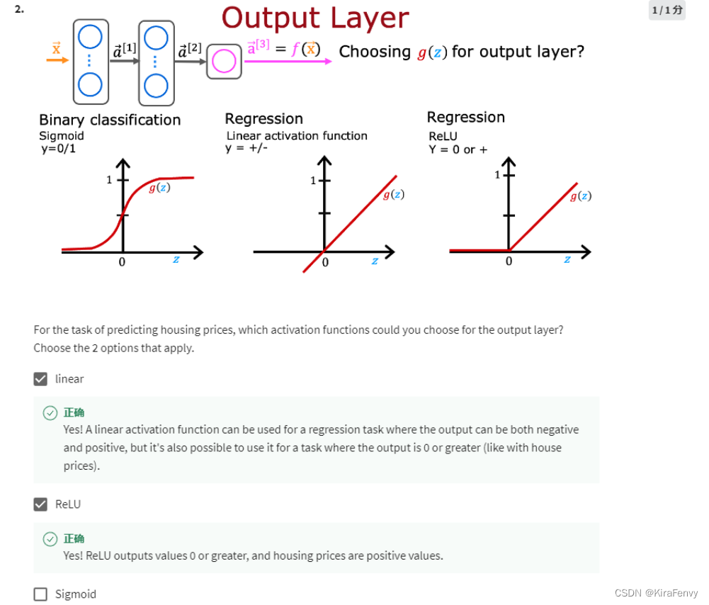
这是输出层的选择， 如果输出必须为0-1（二分类问题），则sigmoid，如果必须非负则ReLU（比如房价），其他回归问题一般就linear

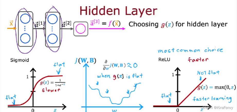
隐藏层的选择：选ReLU比较多（一般都是relu），因为运算速度快，梯度下降速度快，尽量别用linear激活函数，这样跟线性回归没区别

为什么需要激活函数：激活函数决定了，一个神经元是否应该通过加权求和并添加偏差而被激活。激活函数的目的是为神经元添加非线形的输入。一个没有激活函数的神经网络就只是一个线性回归模型，非线形的激活函数能够增加非线性的变换到输入中，使得它能够学习和表现更复杂的任务。

3.使用

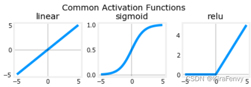
3.1 可视化

def plt_act_trio():
    X = np.linspace(-5,5,100)
    fig,ax = plt.subplots(1,3, figsize=(6,2))
    widgvis(fig)
    ax[0].plot(X,tf.keras.activations.linear(X))
    ax[0].axvline(0, lw=0.3, c="black")
    ax[0].axhline(0, lw=0.3, c="black")
    ax[0].set_title("linear")
    ax[1].plot(X,tf.keras.activations.sigmoid(X))
    ax[1].axvline(0, lw=0.3, c="black")
    ax[1].axhline(0, lw=0.3, c="black")
    ax[1].set_title("sigmoid")
    ax[2].plot(X,tf.keras.activations.relu(X))
    ax[2].axhline(0, lw=0.3, c="black")
    ax[2].axvline(0, lw=0.3, c="black")
    ax[2].set_title("relu")
    fig.suptitle("Common Activation Functions", fontsize=14)
    fig.tight_layout(pad=0.2)
    plt.show()
plt_act_trio()

3.2 载入数据

X = np.random.rand(300, 2)
y = np.sqrt( X[:,0]**2 + X[:,1]**2 ) < 0.6
#y = np.logical_and( X[:,0] < 0.5, X[:,1] < 0.5 ).astype(int)

3.3 模型构建

model = Sequential(
    [ 
        Dense(2,activation="relu",    name = 'l1'),
        Dense(1,activation="sigmoid", name = 'l2')
    ]
)

model.compile(
    loss=tf.keras.losses.MeanSquaredError(),
    optimizer=tf.keras.optimizers.Adam(0.01),
)

model.fit(
    X,y,
    epochs=150
)

绘图函数的代码

def plt_mc_data(ax, X, y, classes,  class_labels=None, map=plt.cm.Paired, 
                legend=False, size=50, m='o', equal_xy = False):
    """ Plot multiclass data. Note, if equal_xy is True, setting ylim on the plot may not work """
    for i in range(classes):
        idx = np.where(y == i)
        col = len(idx[0])*[i]
        label = class_labels[i] if class_labels else "c{}".format(i)
        ax.scatter(X[idx, 0], X[idx, 1],  marker=m,
                    c=col, vmin=0, vmax=map.N, cmap=map,
                    s=size, label=label)
    if legend: ax.legend()
    if equal_xy: ax.axis("equal")

def plt_mc(X_train,y_train,classes):
    css = np.unique(y_train)
    fig,ax = plt.subplots(1,1,figsize=(3,3))
    fig.canvas.toolbar_visible = False
    fig.canvas.header_visible = False
    fig.canvas.footer_visible = False
    plt_mc_data(ax, X_train,y_train,classes, map=dkcolors_map, legend=True, size=10, equal_xy = False)
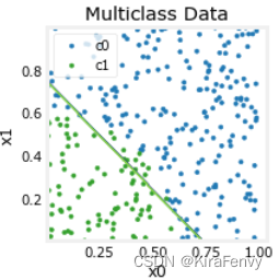
    ax.set_title("Multiclass Data")
    ax.set_xlabel("x0")
    ax.set_ylabel("x1")
    return(ax)
    
def plot_cat_decision_boundary_mc(ax, X, predict , class_labels=None, legend=False, vector=True):

    # create a mesh to points to plot
    x_min, x_max = X[:, 0].min(), X[:, 0].max()
    y_min, y_max = X[:, 1].min(), X[:, 1].max()
    h = max(x_max-x_min, y_max-y_min)/200
    xx, yy = np.meshgrid(np.arange(x_min, x_max, h),
                         np.arange(y_min, y_max, h))
    points = np.c_[xx.ravel(), yy.ravel()]
    #print("points", points.shape)
    #print("xx.shape", xx.shape)

    #make predictions for each point in mesh
    if vector:
        Z = predict(points)
    else:
        Z = np.zeros((len(points),))
        for i in range(len(points)):
            Z[i] = predict(points[i].reshape(1,2))
    Z = Z.reshape(xx.shape)

    #contour plot highlights boundaries between values - classes in this case
    ax.contour(xx, yy, Z, linewidths=1) 
    #ax.axis('tight')

调用并输出结果

ax = plt_mc(X,y,2,)
predict = lambda  x: (model.predict(x) > 0.5).astype(int)
plot_cat_decision_boundary_mc(ax, X, predict, legend = True, vector=True)

下面显示的是在不同层的参数变化

l1 = model.get_layer("l1")
W1,b1 = l1.get_weights()
l2 = model.get_layer("l2")
W2,b2 = l2.get_weights()
print(W1,b1)
print(W2,b2)

[[ 2.74 -1.  ]
 [ 2.7   0.24]] [-1.49 -0.21]
[[-4.95]
 [ 0.88]] [2.61]

4.课后题

1. sigmoid函数适合用在二分类问题
   
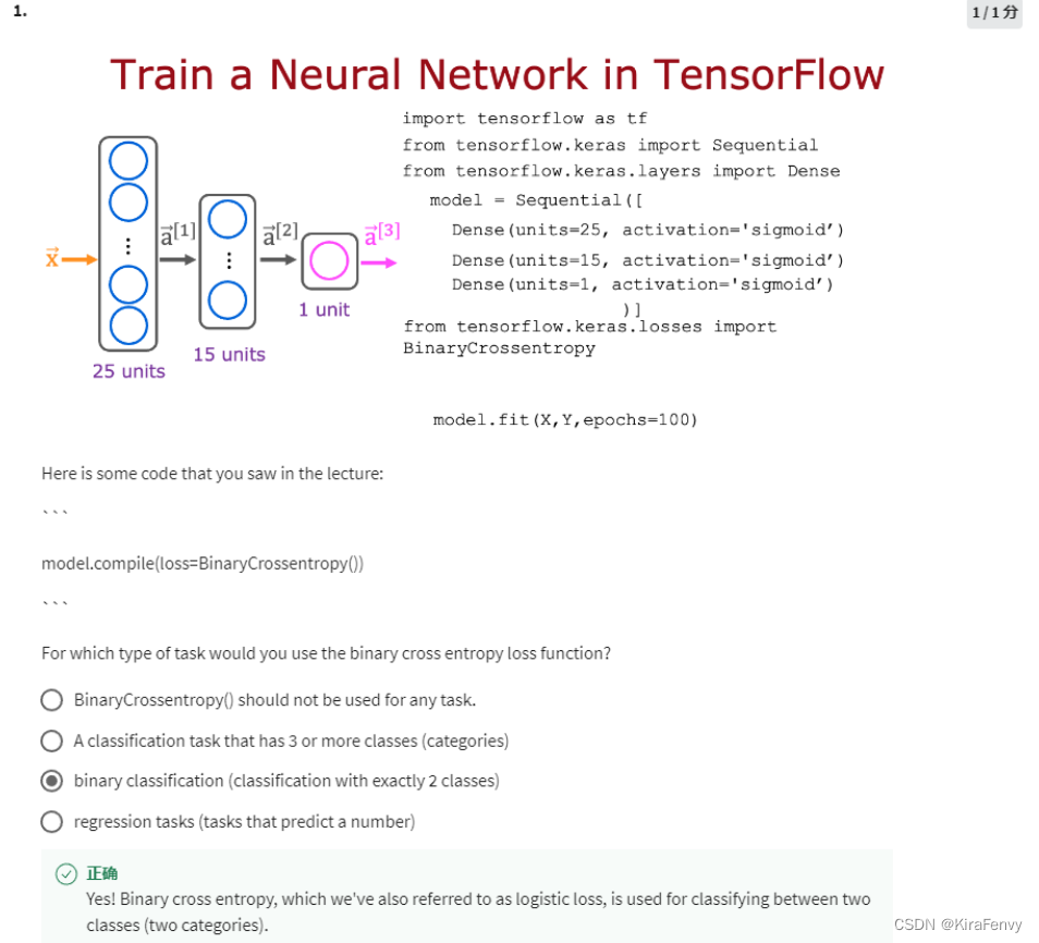
2. 最常用的激活函数就是ReLU函数
   
3. 房价预测是回归问题，不适合使用sigmoid函数

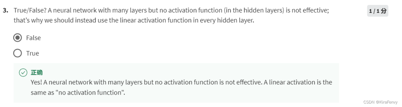
4. 一个神经网络有再多层，没有激活函数是没用的，比如“linear function”实际上就是不做处理