激活函数层 && 神经网络的基本组成 && Sigmoid、ReLU及Softmax函数

Flying Bulldog

已于 2022-05-25 23:43:00 修改

阅读量3.9k

点赞数 8

分类专栏：搭建神经网络 Pytorch_python 文章标签：神经网络深度学习 cnn python pytorch

于 2022-05-25 23:40:38 首次发布

本文链接：https://blog.csdn.net/qq_54185421/article/details/124975832

版权

Pytorch_python 同时被 2 个专栏收录

18 篇文章 5 订阅

订阅专栏

搭建神经网络

5 篇文章 0 订阅

订阅专栏

神经网络如果仅仅是由线性的卷积运算堆叠组成，则其无法形成复杂的表达空间，也就很难提取出高语义的信息，因此还需要加入非线性的映射，又称为激活函数，可以逼近任意的非线性函数，以提升整个神经网络的表达能力。

在物体检测任务中，常用的激活函数有Sigmoid、 ReLU及Softmax函数。

一、常见的激活函数

（1）Sigmoid函数

Sigmoid型函数又称为Logistic函数，模拟了生物的神经元特性，即当神经元获得的输入信号累计超过一定的阈值后，神经元被激活而处于兴奋状态，否则处于抑制状态。表达式如下所示：

Sigmoid函数曲线与梯度曲线如图1所示。可以看到，Sigmoid函数将特征压缩到了(0,1)区间，0端对应抑制状态，而1对应激活状态，中间部分梯度较大。

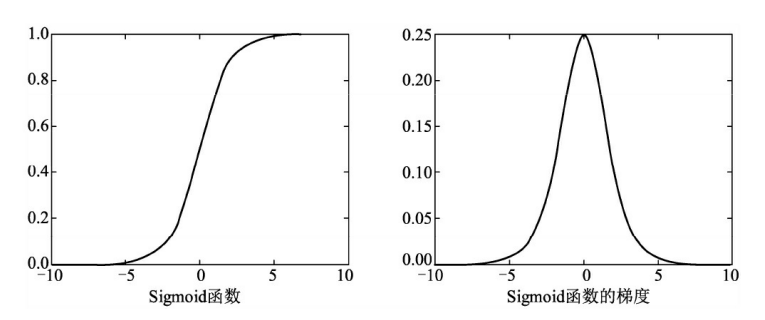
图1 Sigmoid函数及其梯度曲线

Sigmoid函数可以用来做二分类，但其计算量较大，并且容易出现梯度消失现象。从曲线图（图1）中可以看出，在Sigmoid函数两侧的特征导数接近于0，这将导致在梯度反传时损失的误差难以传递到前面的网络层（因为根据链式求导，梯度接近于0）。

（2）ReLU函数

为了缓解梯度消失现象，修正线性单元（Rectified Linear Unit， ReLU）被引入到神经网络中。由于其优越的性能与简单优雅的实现， ReLU已经成为目前卷积神经网络中最为常用的激活函数之一。ReLU函数的表达式如下所示。

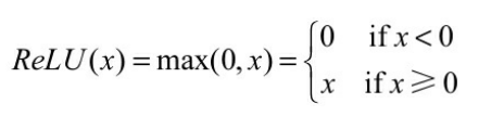
ReLU函数及其梯度曲线如图2 所示。可以看出，在小于0的部分，值与梯度皆为0，而在大于0的部分中导数保持为1，避免了Sigmoid函数中梯度接近于0导致的梯度消失问题。

图2 ReLU函数及其梯度曲线

ReLU函数计算简单，收敛快，并在众多卷积网络中验证了其有效性。

（3）Leaky ReLU函数

ReLU激活函数虽然高效，但是其将负区间所有的输入都强行置为 0，Leaky ReLU函数优化了这一点，在负区间内避免了直接置0，而是赋予很小的权重，其函数表达式如下所示。

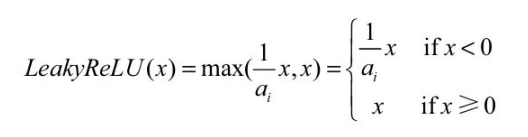
以上公式中的 ai 代表权重，即小于0的值被缩小的比例。Leaky ReLU的函数曲线如图3 所示。

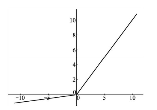
图3 Leaky ReLU函数曲线

虽然从理论上讲，Leaky ReLU函数的使用效果应该要比ReLU函数好，但是从大量实验结果来看并没有看出其效果比ReLU好。此外，对于ReLU函数的变种，除了Leaky ReLU函数之外，还有PReLU和RReLU 函数等，这里不做详细介绍。

（4）Softmax函数

在物体检测中，通常需要面对多物体分类问题，虽然可以使用 Sigmoid函数来构造多个二分类器，但比较麻烦，多物体类别较为常用的分类器是Softmax函数。

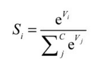
在具体的分类任务中，Softmax函数的输入往往是多个类别的得分，输出则是每一个类别对应的概率，所有类别的概率取值都在0~1之间，且和为1。Softmax函数的表达式如下所示，其中，Vi表示第i 个类别的得分，C代表分类的类别总数，输出Si为第i个类别的概率。

二、Pytorch官方文件激活函数总结

（1）涉及的激活函数，以及公式

nn.ReLU # f(x)= max(0, x)
nn.ReLU6 # f(x) = min(max(0,x), 6)
nn.ELU # f(x) = max(0,x) + min(0, alpha * (e^x - 1))
nn.PReLU # f(x) = max(0,x) + a * min(0,x)
nn.LeakyReLU # f(x) = max(0, x) + {negative_slope} * min(0, x)
nn.Threshold # y=x,if x>=threshold y=value,if x<threshold
nn.Hardtanh # f(x)=+1,if x>1; f(x)=−1,if x<−1; f(x)=x,otherwise
nn.Sigmoid # f(x)=1/(1+e−x)
nn.Tanh # f(x)=ex−e−xex+ex
nn.LogSigmoid # f(x) = log( 1 / ( 1 + e^{-x}))
nn.Softplus # f(x)=1beta∗log(1+e(beta∗xi))
nn.Softshrink # f(x)=x−lambda,if x>lambda f(x)=x+lambda, if x<−lambda f(x)=0,otherwise
nn.Softsign # f(x) = x / (1 + |x|)
nn.Tanhshrink # f(x)=x−Tanh(x)
nn.Softmin # fi(x)=e(−xi−shift)∑je(−xj−shift),shift=max(xi)
nn.Softmax # fi(x)=e(xi−shift)∑je(xj−shift),shift=max(xi)
nn.LogSoftmax # fi(x)=loge(xi)a,a=∑je(xj)

（2）代码示例（含注释）

import torch
import torch.nn as nn
from torch import autograd

# torch.nn.ReLU(inplace=False)
# 对输入运用修正线性单元函数${ReLU}(x)= max(0, x)$，
# 参数： inplace-选择是否进行覆盖运算
m = nn.ReLU()
input = autograd.Variable(torch.randn(2))
print(input)
print(m(input))

# torch.nn.ReLU6(inplace=False)
# 对输入的每一个元素运用函数${ReLU6}(x) = min(max(0,x), 6)$，
m = nn.ReLU6()
input = autograd.Variable(torch.randn(2))
print(input)
print(m(input))

# torch.nn.ELU(alpha=1.0, inplace=False)
# 对输入的每一个元素运用函数$f(x) = max(0,x) + min(0, alpha * (e^x - 1))$
m = nn.ELU()
input = autograd.Variable(torch.randn(2))
print(input)
print(m(input))

# torch.nn.PReLU(num_parameters=1, init=0.25)
# 对输入的每一个元素运用函数$PReLU(x) = max(0,x) + a * min(0,x)$，a 是一个可学习参数。
# 当没有声明时，nn.PReLU()在所有的输入中只有一个参数 a；
# 如果是 nn.PReLU(nChannels)，a 将应用到每个输入。
# 注意：当为了表现更佳的模型而学习参数 a 时不要使用权重衰减（weight decay）
# 参数：
# num_parameters：需要学习的 a 的个数，默认等于 1
# init：a 的初始值，默认等于 0.25
m = nn.PReLU()
input = autograd.Variable(torch.randn(2))
print(input)
print(m(input))

# torch.nn.LeakyReLU(negative_slope=0.01, inplace=False)
# 对输入的每一个元素运用$f(x) = max(0, x) + {negative_slope} * min(0, x)$
# 参数：
# negative_slope：控制负斜率的角度，默认等于 0.01
# inplace-选择是否进行覆盖运算
m = nn.LeakyReLU(0.1)
input = autograd.Variable(torch.randn(2))
print(input)
print(m(input))

import torch
import torch.nn as nn
from torch import autograd

# torch.nn.Threshold(threshold, value, inplace=False)
# Threshold 定义：y=x,if x>=threshold y=value,if x<threshold
# 参数：
# threshold：阈值
# value：输入值小于阈值则会被 value 代替
# inplace：选择是否进行覆盖运算
m = nn.Threshold(0.1, 20)
input = autograd.Variable(torch.Tensor([0.26, 0]))
print(input)
print(m(input))

# torch.nn.Hardtanh(min_value=-1, max_value=1, inplace=False)
# 对每个元素，f(x)=+1,if x>1; f(x)=−1,if x<−1; f(x)=x,otherwise
# 线性区域的范围[-1,1]可以被调整
# 参数：
# min_value：线性区域范围最小值
# max_value：线性区域范围最大值
# inplace：选择是否进行覆盖运算
m = nn.Hardtanh()
input = autograd.Variable(torch.Tensor([0.2, -3, 5]))
print(input)
print(m(input))

# torch.nn.Sigmoid
# 对每个元素运用 Sigmoid 函数，Sigmoid 定义如下：f(x)=1/(1+e−x)
m = nn.Sigmoid()
input = autograd.Variable(torch.Tensor([0, 3, 10]))
print(input)
print(m(input))

# torch.nn.Tanh
# 对输入的每个元素，f(x)=ex−e−xex+ex
m = nn.Tanh()
input = autograd.Variable(torch.randn(2))
print(input)
print(m(input))

# torch.nn.LogSigmoid
# 对输入的每个元素，$LogSigmoid(x) = log( 1 / ( 1 + e^{-x}))$
m = nn.LogSigmoid()
input = autograd.Variable(torch.randn(2))
print(input)
print(m(input))

# torch.nn.Softplus(beta=1, threshold=20)
# 对每个元素运用 Softplus 函数，Softplus 定义如下：f(x)=1beta∗log(1+e(beta∗xi))
# Softplus 函数是 ReLU 函数的平滑逼近，Softplus 函数可以使得输出值限定为正数。
# 为了保证数值稳定性，线性函数的转换可以使输出大于某个值。
# 参数：
# beta：Softplus 函数的 beta 值
# threshold：阈值
m = nn.Softplus(beta=2, threshold=10)
m1 = nn.Softplus()
input = autograd.Variable(torch.randn(2))
print(input)
print(m(input))
print(m1(input))

# torch.nn.Softshrink(lambd=0.5)
# 对每个元素运用 Softshrink 函数，Softshrink 函数定义如下：
# f(x)=x−lambda,if x>lambda f(x)=x+lambda,if x<−lambda f(x)=0,otherwise
# 参数：
# lambd：Softshrink 函数的 lambda 值，默认为 0.5
m = nn.Softshrink()
input = autograd.Variable(torch.randn(2))
print(input)
print(m(input))

# torch.nn.Softsign
# $f(x) = x / (1 + |x|)$
m = nn.Softsign()
input = autograd.Variable(torch.Tensor([1, 2]))
print(input)
print(m(input))

# torch.nn.Softshrink(lambd=0.5)
# 对每个元素运用 Tanhshrink 函数，Tanhshrink 函数定义如下：
# Tanhshrink(x)=x−Tanh(x)
m = nn.Tanhshrink()
input = autograd.Variable(torch.randn(2))
m_tanh = nn.Tanh()
print(input)
print(m_tanh(input))
print(m(input))

# torch.nn.Softmin
# 对 n 维输入张量运用 Softmin 函数，将张量的每个元素缩放到（0,1）区间且和为 1。Softmin 函数定义如下：
# fi(x)=e(−xi−shift)∑je(−xj−shift),shift=max(xi)
# dim (int)：计算 Softmin 的维度（因此沿 dim 的每个切片的总和为 1）。
m = nn.Softmin(dim=0)
input = autograd.Variable(torch.randn(2, 3))
print(input)
print(m(input))

# torch.nn.Softmax
# 对 n 维输入张量运用 Softmax 函数，将张量的每个元素缩放到（0,1）区间且和为 1。
# Softmax 函数定义如下：fi(x)=e(xi−shift)∑je(xj−shift),shift=max(xi)
# 返回结果是一个与输入维度相同的张量，每个元素的取值范围在（0,1）区间。
m = nn.Softmax(dim=0)
input = autograd.Variable(torch.randn(2, 3))
print(input)
print(m(input))

# torch.nn.LogSoftmax
# 对 n 维输入张量运用 LogSoftmax 函数，LogSoftmax 函数定义如下：
# fi(x)=loge(xi)a,a=∑je(xj)
m = nn.LogSoftmax(dim=0)
input = autograd.Variable(torch.randn(2, 3))
print(input)
print(m(input))

>>>本文参考：Pytoch官方文件 &&《深度学习之PyTorch物体检测实战》

>>>如有疑问，欢迎评论区一起探讨

Flying Bulldog

关注

8
点赞
踩
28

收藏

觉得还不错? 一键收藏
打赏
0
评论
激活函数层 && 神经网络的基本组成 && Sigmoid、ReLU及Softmax函数

神经网络如果仅仅是由线性的卷积运算堆叠组成，则其无法形成复杂的表达空间，也就很难提取出高语义的信息，因此还需要加入非线性的映射，又称为激活函数，可以逼近任意的非线性函数，以提升整个神经网络的表达能力。在物体检测任务中，常用的激活函数有Sigmoid、 ReLU及Softmax函数。目录一、常见的激活函数（1）Sigmoid函数（2）ReLU函数（3）Leaky ReLU函数（4）Softmax函数二、Pytorch官方文件激活函数总结（1）涉及的激活函数，以及公式..
复制链接

扫一扫