


CW算法
1 引言
对抗攻击的方式主要分为三大类,第一种是基于梯度迭代的攻击方式比如FGSM,PGD,MIM;第二种是基于GAN 的攻击方式,比如AdvGAN,AdvGAN++,AdvFaces。还有一种攻击方式为基于优化的攻击方式,它的代表就是本文CW的攻击。CW攻击产生的对抗样本所加入的扰动,几乎是人眼察觉不出来的,反观,FGSM和PGD生成的对抗样本所生成的扰动比较糊,而且CW的攻击效果更加好,在加有蒸馏防御的分类模型中,CW攻击依然可以高效地攻击成功。
生成样本算法都要保证如下两个条件:
1、对抗样本和干净样本的差距应该越小越好。评价指标有 L0,L2,L正无穷
2、对抗样本应该使得模型分类错,且分类错的那一类的置信度应足够的高(有目标攻击)。
条件一,保证了生成样本与原始干净样本尽量的相似。
条件二,保证了生成样本确实能成功攻击模型。
仔细想想,这两个条件是不是就满足了生成样本的全部需求
2 思路跟进
假设输入样本为
x
x
x,扰动为
ε
\varepsilon
ε,
D
D
D为距离地量函数,C为模型分类结果,t为定向攻击标签。将次概括为优化问题,如下
minimize
D
(
x
,
x
+
ϵ
)
s.t.
c
(
x
+
ϵ
)
=
t
x
+
ϵ
∈
[
0
,
1
]
n
\begin{aligned} & \text{minimize} \quad D(x, x + \epsilon) \\ & \text{s.t.} \quad c(x + \epsilon) = t \\ & \quad x + \epsilon \in [0, 1]^n \end{aligned}
minimizeD(x,x+ϵ)s.t.c(x+ϵ)=tx+ϵ∈[0,1]n
然而由于
C
(
x
+
ε
)
=
t
C(x+\varepsilon)=t
C(x+ε)=t是高度非线性的,因此现有的算法都难以直接求解,上面的式子,所以需要选择一种更适合优化的表达方式。即定义一个目标函数
f
f
f,当且仅当
f
(
x
+
ε
)
≤
0
f(x+\varepsilon)\le0
f(x+ε)≤0时,
C
(
x
+
ε
)
=
t
C(x+\varepsilon)=t
C(x+ε)=t。我们可以用如下的一个式子来当做
f
f
f。
f
(
x
′
)
=
(
m
a
x
i
≠
t
(
F
(
x
′
)
i
)
−
F
(
x
′
)
t
)
+
f(x') = (max_{i\ne t}(F(x')_i)-F(x')_t)^+
f(x′)=(maxi=t(F(x′)i)−F(x′)t)+
式中,
t
t
t表示定向攻击标签,
(
∗
)
+
(*)^+
(∗)+表示
m
a
x
(
∗
,
0
)
;
max(*,0);
max(∗,0);,
F
(
x
′
)
i
F(x')_i
F(x′)i表示当神经网络输入为
x
′
x'
x′时,产生类别是
i
i
i的概率;
Z
(
x
′
)
Z(x')
Z(x′)表示softmax层前的输出,即
F
(
x
)
=
s
o
f
t
m
a
x
(
Z
(
x
)
)
F(x)=softmax(Z(x))
F(x)=softmax(Z(x));
l
o
s
s
F
,
t
(
x
′
)
loss_{F,t}(x')
lossF,t(x′)为交叉熵。
上面给出的
f
(
x
)
f(x)
f(x),
m
a
x
i
≠
t
(
F
(
x
′
)
i
)
max_{i\ne t}(F(x')_i)
maxi=t(F(x′)i)表示除了目标类别
t
t
t外,模型当前输入认为最有可能属于类别
i
i
i,输入类别
i
i
i的概率依旧小于类别
t
t
t的概率,认为此时攻击成功。换言之,就是当识别为类别
t
t
t的概率最大时,认为攻击成功。
所以可以对公式进行重新改写。
minimize
D
(
x
,
x
+
ε
)
s.t.
f
(
x
+
ϵ
)
≤
0
x
+
ε
∈
[
0
,
1
]
n
\begin{aligned} & \text{minimize} \quad D(x, x + \varepsilon) \\ & \text{s.t.} \quad f(x + \epsilon) \le 0\\ & \quad x + \varepsilon \in [0, 1]^n \end{aligned}
minimizeD(x,x+ε)s.t.f(x+ϵ)≤0x+ε∈[0,1]n
这个地方应该还是
x
+
ϵ
∈
[
0
,
1
]
n
x + \epsilon \in [0, 1]^n
x+ϵ∈[0,1]n好一点,原书的公式不带上标n,不清楚为什么。
将上述的约束条件转换为目标函数,令距离度量函数
D
D
D为
L
p
L_p
Lp范数,得到以下约束:
m
i
n
∣
∣
δ
∣
∣
p
+
c
f
(
x
+
ε
)
s
.
t
.
x
+
ε
∈
[
0
,
1
]
n
min\quad||\delta||_p+cf(x+\varepsilon)\\ s.t. \quad x+\varepsilon \in [0,1]^n
min∣∣δ∣∣p+cf(x+ε)s.t.x+ε∈[0,1]n
其中的
∣
∣
δ
∣
∣
p
||\delta||_p
∣∣δ∣∣p项即上面式子中的
D
(
x
,
x
+
ε
)
D(x, x + \varepsilon)
D(x,x+ε),这一项代表着对抗样本和原始样本的
L
2
L_2
L2范数距离,也就是扰动,回顾对抗样本生成的目标:“生成样本与原始干净样本尽量的相似”,使这一项最小化,就保证了生成的对抗样本与原始样本尽可能地相似;
c
f
(
x
+
ε
)
cf(x+\varepsilon)
cf(x+ε)表示分类结果越符合目标结果越好,上面给出的
f
(
x
)
f(x)
f(x)中,如果
F
(
x
′
)
t
F(x')_t
F(x′)t越大(即分类为目标类的概率越大),那么
c
f
(
x
+
ε
)
cf(x+\varepsilon)
cf(x+ε)的值越小,也就为了满足生成对抗样本的第二个要求:生成样本确实能成功攻击模型。
由于对抗样本增加、减去剃度之后很容易超出 [ 0 , 1 ] [0,1] [0,1]的范围,为了生成有效的图片,需要对其进行约束,使得 0 ≤ x i + δ i ≤ 1 0\le x_i+\delta_i \le 1 0≤xi+δi≤1。对生成样本进行clip截断就可以将其约束在[0,1]的范围内,我们可以现在只需不断的进行迭代,找到最小值就可以生成对抗样本了。
然而,使用截断的思想,但会使攻击性能下降,CW算法提出的思想,将其映射到tanh空间,为此,CW算法作者引入了新的变量
w
w
w。
x
+
δ
=
1
2
(
t
a
n
h
(
w
)
+
1
)
δ
=
1
2
(
t
a
n
h
(
w
)
+
1
)
−
x
x+\delta = \frac{1}{2}(tanh(w)+1)\\ \delta = \frac{1}{2}(tanh(w)+1)-x
x+δ=21(tanh(w)+1)δ=21(tanh(w)+1)−x
因为tanh函数的值域为 [ − 1 , 1 ] [-1,1] [−1,1],所以 x + δ x+\delta x+δ的取值范围是 [ 0 , 1 ] [0,1] [0,1],这样就满足了约束条件。
下面给出已CW算法的
L
2
L_2
L2范数攻击定义式
m
i
n
i
m
i
z
e
∣
∣
1
2
(
t
a
n
h
(
w
)
+
1
)
−
x
∣
∣
2
2
+
c
f
(
1
2
(
t
a
n
h
(
w
)
+
1
)
)
f
(
x
′
)
=
m
a
x
(
m
a
x
{
Z
(
x
′
)
i
:
i
≠
t
}
−
Z
(
x
′
)
t
,
−
K
)
minimize \quad ||\frac{1}{2}(tanh(w)+1)-x||_2^2+cf(\frac{1}{2}(tanh(w)+1))\\ f(x')=max(max\{ Z(x')_i:i\ne t \}-Z(x')_t, -K)
minimize∣∣21(tanh(w)+1)−x∣∣22+cf(21(tanh(w)+1))f(x′)=max(max{Z(x′)i:i=t}−Z(x′)t,−K)
f f f在式中添加了参数 K K K,改参数能够控制误分类发生的置信度。保证找到的对抗样本 x ′ x' x′能够以较好的置信度被误分为类别 t t t。最初我自己看的时候不好理解,下面给出两个式子大家理解一下。
2.1 对于K的理解
先看第一种:
假设现在有
K
=
0.2
K=0.2
K=0.2,且假设此时
m
a
x
{
Z
(
x
′
)
i
:
i
≠
t
}
−
Z
(
x
′
)
t
≤
−
K
max\{ Z(x')_i:i\ne t \}-Z(x')_t \le -K
max{Z(x′)i:i=t}−Z(x′)t≤−K,即
f
(
x
′
)
=
m
a
x
(
m
a
x
{
Z
(
x
′
)
i
:
i
≠
t
}
−
Z
(
x
′
)
t
,
−
K
)
=
−
K
f(x')=max(max\{ Z(x')_i:i\ne t \}-Z(x')_t, -K)=-K
f(x′)=max(max{Z(x′)i:i=t}−Z(x′)t,−K)=−K,那么式可以变成
m
i
n
i
m
i
z
e
∣
∣
1
2
(
t
a
n
h
(
w
)
+
1
)
−
x
∣
∣
2
2
+
c
∗
(
−
0.2
)
f
(
x
′
)
=
−
K
=
−
0.2
minimize \quad ||\frac{1}{2}(tanh(w)+1)-x||_2^2+c*(-0.2)\\ f(x')=-K=-0.2
minimize∣∣21(tanh(w)+1)−x∣∣22+c∗(−0.2)f(x′)=−K=−0.2
再看第二种:
假设现在有
K
=
0.8
K=0.8
K=0.8,且假设此时
m
a
x
{
Z
(
x
′
)
i
:
i
≠
t
}
−
Z
(
x
′
)
t
≤
−
K
max\{ Z(x')_i:i\ne t \}-Z(x')_t \le -K
max{Z(x′)i:i=t}−Z(x′)t≤−K,即
f
(
x
′
)
=
m
a
x
(
m
a
x
{
Z
(
x
′
)
i
:
i
≠
t
}
−
Z
(
x
′
)
t
,
−
K
)
=
−
K
f(x')=max(max\{ Z(x')_i:i\ne t \}-Z(x')_t, -K)=-K
f(x′)=max(max{Z(x′)i:i=t}−Z(x′)t,−K)=−K,那么式可以变成
m
i
n
i
m
i
z
e
∣
∣
1
2
(
t
a
n
h
(
w
)
+
1
)
−
x
∣
∣
2
2
+
c
∗
(
−
0.8
)
f
(
x
′
)
=
−
K
=
−
0.8
minimize \quad ||\frac{1}{2}(tanh(w)+1)-x||_2^2+c*(-0.8)\\ f(x')=-K=-0.8
minimize∣∣21(tanh(w)+1)−x∣∣22+c∗(−0.8)f(x′)=−K=−0.8
差别就在于,第一种情况的
f
(
x
′
)
f(x')
f(x′)值更小,因此优化过程更倾向于最小化数据项的平方误差
∣
∣
1
2
(
t
a
n
h
(
w
)
+
1
)
−
x
∣
∣
2
2
||\frac{1}{2}(tanh(w)+1)-x||_2^2
∣∣21(tanh(w)+1)−x∣∣22。因此,它可能会导致更小的
∣
∣
1
2
(
t
a
n
h
(
w
)
+
1
)
−
x
∣
∣
2
2
||\frac{1}{2}(tanh(w)+1)-x||_2^2
∣∣21(tanh(w)+1)−x∣∣22 值,即更接近数据
x
x
x 的拟合结果。可以理解为K越大,置信度越大。
说白了,我们控制想要达到的置信度,然后在此置信度限定下,寻找最小距离和最大置信度的最优解,设置K值就是选择我们希望项更优,K越小,那么就会偏向于使距离更小,K越大置信度越高,不能保证说距离就一定比较大,但是从主观上来说我们更加关注置信度的好坏,而不太关心距离(感觉可以看做权重)。
2.2 手稿模拟
现在我们的思路已经很清楚了,CW算法本身是一个基于优化的对抗样本算法,我们要在迭代中不断地优化扰动的距离和置信度。但尽情上面的公式要写出代码好像不太容易,我们理解了基本思路之后,再看一遍形式化的定义,帮助我们更好理解算法,以便写出代码。这部分内容主要参考:https://blog.csdn.net/weixin_41466575/article/details/117738731
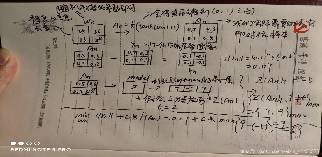
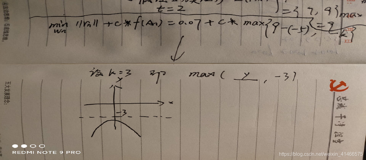
A
n
=
1
2
(
t
a
n
h
(
W
n
)
+
1
)
r
n
=
A
n
−
X
n
m
i
n
i
m
i
z
e
∣
∣
r
n
∣
∣
2
2
+
c
∗
f
(
A
n
)
f
(
A
n
)
=
m
a
x
(
m
a
x
{
Z
(
A
n
)
i
:
i
≠
t
}
−
Z
(
A
n
)
t
,
−
K
)
A_n = \frac{1}{2}(tanh(W_n)+1)\\ r_n = A_n - X_n\\ minimize \quad ||r_n||_2^2+c*f(A_n)\\ f(A_n)=max(max\{ Z(A_n)_i:i\ne t \}-Z(A_n)_t, -K)
An=21(tanh(Wn)+1)rn=An−Xnminimize∣∣rn∣∣22+c∗f(An)f(An)=max(max{Z(An)i:i=t}−Z(An)t,−K)
W
n
W_n
Wn表示优化参数,
A
n
A_n
An表示对抗样本,
X
n
X_n
Xn表示干净样本,
r
n
r_n
rn代表对抗样本与干净样本的L2距离;c为超参数,用来权衡两个loss之间的关系;
Z
(
A
n
)
t
Z(A_n)_t
Z(An)t表示对抗样本输入模型后,未经过softmax层输出结果的第t个类别之;K就是置信度;K越大,模型分类到目标类别的概率越大。
3 torch代码实现
这里我之前用腾讯安全朱雀实验室的《AI安全》学了FGSM算法,直接使用他的实例代码中的MNIST模型来进行CW攻击。
# -*- coding: utf-8 -*-
from __future__ import print_function
import torch
import torch.nn as nn
import torch.nn.functional as F
import torch.optim as optim
from torchvision import datasets, transforms
import numpy as np
import matplotlib.pyplot as plt

# NOTE: This is a hack to get around "User-agent" limitations when downloading MNIST datasets
#       see, https://github.com/pytorch/vision/issues/3497 for more information
from six.moves import urllib
opener = urllib.request.build_opener()
opener.addheaders = [('User-agent', 'Mozilla/5.0')]
urllib.request.install_opener(opener)

epsilons = [0, .05, .1, .15, .2, .25, .3]
pretrained_model = "data/lenet_mnist_model.pth"
use_cuda=True


# LeNet Model definition
class Net(nn.Module):
    def __init__(self):
        super(Net, self).__init__()
        self.conv1 = nn.Conv2d(1, 10, kernel_size=5)
        self.conv2 = nn.Conv2d(10, 20, kernel_size=5)
        self.conv2_drop = nn.Dropout2d()
        self.fc1 = nn.Linear(320, 50)
        self.fc2 = nn.Linear(50, 10)

    def forward(self, x):
        x = F.relu(F.max_pool2d(self.conv1(x), 2))
        x = F.relu(F.max_pool2d(self.conv2_drop(self.conv2(x)), 2))
        x = x.view(-1, 320)
        x = F.relu(self.fc1(x))
        x = F.dropout(x, training=self.training)
        x = self.fc2(x)
        return F.log_softmax(x, dim=1)

# MNIST Test dataset and dataloader declaration
test_loader = torch.utils.data.DataLoader(
    datasets.MNIST('./data', train=False, download=True, transform=transforms.Compose([
            transforms.ToTensor(),
            ])),
        batch_size=1, shuffle=True)

# Define what device we are using
print("CUDA Available: ",torch.cuda.is_available())
device = torch.device("cuda" if (use_cuda and torch.cuda.is_available()) else "cpu")

# Initialize the network
model = Net().to(device)

# Load the pretrained model
model.load_state_dict(torch.load(pretrained_model, map_location='cpu'))

# Set the model in evaluation mode. In this case this is for the Dropout layers
model.eval()


# 初始化分类器
classifier = Net()

# 定义对抗样本生成器
class CWAttack:
    def __init__(self, classifier, c=1, kappa=0, learning_rate=0.01, num_iterations=1000):
        self.classifier = classifier  # 分类器
        self.c = c  # CW算法中的c参数
        self.kappa = kappa  # CW算法中的kappa参数
        self.learning_rate = learning_rate  # 优化器的学习率
        self.num_iterations = num_iterations  # 迭代次数
        self.clip_min = 0
        self.clip_max = 1

    def generate(self, x, target):
        #x_adv = Variable(x.data, requires_grad=True)                     # 对抗样本微调
        x_adv = x.clone().detach().requires_grad_(True)  # 对抗样本微调
        # x_adv = nn.Variable(torch.rand(x.size()), requires_grad=True)       # 随机的生成初始样本
        optimizer = optim.Adam([x_adv], lr=self.learning_rate)  # 优化器

        for i in range(self.num_iterations):
            optimizer.zero_grad()  # 清空梯度
            output = self.classifier(x_adv)  # 分类器的输出

            # 如果已经成功生成对抗样本,则退出循环
            if self.is_adversarial(output, target):
                break

            # 没有成功预测,开始优化
            loss = self.cw_loss(output, target, x, x_adv)  # 计算CW损失
            loss.backward()  # 反向传播
            optimizer.step()  # 优化像素值

            # 限制像素值在0到1之间
            # x_adv.data = torch.clamp(x_adv.data, 0, 1)
            # 使用梯度更新对抗样本
            x_adv.data = (torch.tanh(x_adv.data) + 1) / 2 * (self.clip_max - self.clip_min) + self.clip_min


        return x_adv

    def cw_loss(self, output, target, x, x_adv):
        # 计算距离项
        distance = torch.norm(x_adv - x, p=2)           # 计算L2范数,即距离

        # 计算分类误差项
        if self.kappa == 0:
            # print(output)
            target_tensor = torch.tensor([target]).to(output.device) # 将target转换为张量
            # print(target_tensor)
            loss = nn.functional.nll_loss(output, target_tensor)  # 交叉熵损失

        else:
            target_one_hot = torch.zeros(output.size())
            target_one_hot[0][target] = 1  # 将目标类的one-hot编码设为1
            other_classes = torch.masked_select(output, target_one_hot.byte())  # 获取非目标类的输出
            top_other_classes = other_classes.topk(k=self.kappa)[0]  # 获取非目标类中前k个最大的输出
            loss = torch.clamp(output[0][target] - top_other_classes[-1], min=-self.c)  # 计算CW损失

        # 组合距离项和分类误差项
        return loss + distance

    def is_adversarial(self, output, target):
        return torch.argmax(output.data) == target  # 判断是否生成了对抗样本,即是否将分类器输出的最大值设为目标类

target = 9
# 定义对抗样本生成器
attack = CWAttack(classifier)
original = 0

# 测试对抗样本生成器
count = 0
for i,j in test_loader:
    if count == 100:
        break
    original = i
    # print(j[0])
    if j[0] == target:
        continue

    x_adv = attack.generate(i, target)
    result = x_adv.clone().detach().requires_grad_(False)
    dif = x_adv - result
    # plt.imsave("./result/{}with{}to{}.png".format(count, j[0], target), result.squeeze(), cmap="gray")
    count += 1
    cnt = 1
    plt.subplot(1, 2, cnt)
    plt.imshow(original.squeeze(), cmap='gray')
    plt.title('Original Image')
    cnt += 1
    plt.subplot(1, 2, cnt)
    plt.imshow(result.squeeze(), cmap='gray')
    plt.title('Adversarial Image')
    cnt += 1
    plt.subplot(1, 2, cnt)
    plt.imshow(dif.squeeze(), cmap='gray')
    #axs[1].imshow(x_adv, cmap='gray')
    plt.title('Adversarial Image')
    plt.savefig("./result/{}with{}to{}.png".format(count, j[0], target))
4 总结
CW是一个基于优化的攻击,主要调节的参数是c和k,看你自己的需要了。它的优点在于,可以调节置信度,生成的扰动小,可以破解很多的防御方法,缺点是,很慢。


 4491
4491

 被折叠的 条评论
为什么被折叠?
被折叠的 条评论
为什么被折叠?
 到【灌水乐园】发言


