


1 笔者言
- 虽说标题有DeepFool原理,但能力有限,这个我确实讲不清楚。与FGSM,BIM,MIM,CW等生成对抗样本的方法相比,deepfool是最难的了。给你推荐一个我看懂了的文章,但切记,想要真正明白deepfool的原理,就一定要耐下性子认真看,还要多动笔画示意图。言至此,传送门
- 本文主要讲解代码,完成生成deepfool对抗样本的完整过程。直接复制代码就能跑。相信我,不骗你。
- 使用pytorch实现deepfool。pytorch不会?跳转
- CVPR 2016 论文地址
2 coding
- 实验步骤:
- 训练一个简单模型(mnist手写数字分类任务)
- 通过该模型生成对抗样本
- 测试生成对抗样本的鲁棒性
- 可视化展示对抗样本效果
2.1 训练模型
from __future__ import print_function
import torch
import torch.nn as nn
import torch.nn.functional as F
import torch.optim as optim
from torchvision import datasets, transforms
import numpy as np
import matplotlib.pyplot as plt
from tqdm import tqdm

# 加载mnist数据集
test_loader = torch.utils.data.DataLoader(
    datasets.MNIST('../data', train=False, download=True, transform=transforms.Compose([
            transforms.ToTensor(),
            ])),
        batch_size=10, shuffle=True)
train_loader = torch.utils.data.DataLoader(
    datasets.MNIST('../data', train=True, download=True, transform=transforms.Compose([
            transforms.ToTensor(),
            ])),
        batch_size=10, shuffle=True)

# 超参数设置
batch_size = 10
epoch = 1
learning_rate = 0.001
# 生成对抗样本的个数
adver_nums = 1000


# LeNet Model definition
class Net(nn.Module):
    def __init__(self):
        super(Net, self).__init__()
        self.conv1 = nn.Conv2d(1, 10, kernel_size=5)
        self.conv2 = nn.Conv2d(10, 20, kernel_size=5)
        self.conv2_drop = nn.Dropout2d()
        self.fc1 = nn.Linear(320, 50)
        self.fc2 = nn.Linear(50, 10)

    def forward(self, x):
        x = F.relu(F.max_pool2d(self.conv1(x), 2))
        x = F.relu(F.max_pool2d(self.conv2_drop(self.conv2(x)), 2))
        x = x.view(-1, 320)
        x = F.relu(self.fc1(x))
        x = F.dropout(x, training=self.training)
        x = self.fc2(x)
        return F.log_softmax(x, dim=1)

# 选择设备
device = torch.device("cuda" if (torch.cuda.is_available()) else "cpu")

# 初始化网络,并定义优化器
simple_model = Net().to(device)
optimizer1 = torch.optim.SGD(simple_model.parameters(),lr = learning_rate,momentum=0.9)
print (simple_model)
Output:
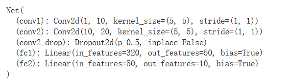
- 如上代码,下载数据,设置超参数以及构建模型
- 如下代码,开始训练模型,并进行测试,观察模型准确率
# 训练模型
def train(model,optimizer):
  for i in range(epoch):
    for j,(data,target) in tqdm(enumerate(train_loader)):
      data = data.to(device)
      target = target.to(device)
      logit = model(data)
      loss = F.nll_loss(logit,target)
      model.zero_grad()
      # 如下:因为其中的loss是单个tensor就不能用加上一个tensor的维度限制
      loss.backward()
      # 如下有两种你形式表达,一种是原生,一种是使用optim优化函数直接更新参数
      # 为什么原生的训练方式没有效果???代表参数没有更新,就离谱。
      # 下面的detach与requires_grad_有讲究哦,终于明白了;但是为什么下面代码不能work还是没搞懂
      # for params in model.parameters():
      #   params = (params - learning_rate * params.grad).detach().requires_grad_()
      optimizer.step()
      if j % 1000 == 0:
        print ('第{}个数据,loss值等于{}'.format(j,loss))
train(simple_model,optimizer1)

# eval eval ,老子被你害惨了
# 训练完模型后,要加上,固定DROPOUT层
simple_model.eval()

# 模型测试
def test(model,name):
  correct_num = torch.tensor(0).to(device)
  for j,(data,target) in tqdm(enumerate(test_loader)):
    data = data.to(device)
    target = target.to(device)
    logit = model(data)
    pred = logit.max(1)[1]
    num = torch.sum(pred==target)
    correct_num = correct_num + num
  print (correct_num)
  print ('\n{} correct rate is {}'.format(name,correct_num/10000))
test(simple_model,'simple model')
Output:

2.2 DeepFool对抗样本生成
import numpy as np
from torch.autograd import Variable
import torch as torch
import copy
# 下面导入的类是很早版本的,现在版本已经没有了
# from torch.autograd.gradcheck import zero_gradients


def deepfool(image, net, num_classes=10, overshoot=0.02, max_iter=100):
    is_cuda = torch.cuda.is_available()
    if is_cuda:
        # print("Using GPU")
        image = image.cuda()
        net = net.cuda()

    f_image = net.forward(Variable(image[None, :, :, :], requires_grad=True)).data.cpu().numpy().flatten()
    I = (np.array(f_image)).flatten().argsort()[::-1]

    I = I[0:num_classes]
    label = I[0]

    input_shape = image.cpu().numpy().shape
    pert_image = copy.deepcopy(image)
    w = np.zeros(input_shape)
    r_tot = np.zeros(input_shape)

    loop_i = 0

    x = Variable(pert_image[None, :], requires_grad=True)
    fs = net.forward(x)
    fs_list = [fs[0,I[k]] for k in range(num_classes)]
    k_i = label

    while k_i == label and loop_i < max_iter:

        pert = np.inf
        fs[0, I[0]].backward(retain_graph=True)
        grad_orig = x.grad.data.cpu().numpy().copy()

        for k in range(1, num_classes):
            if x.grad is not None:
              x.grad.zero_()

            fs[0, I[k]].backward(retain_graph=True)
            cur_grad = x.grad.data.cpu().numpy().copy()

            # set new w_k and new f_k
            w_k = cur_grad - grad_orig
            f_k = (fs[0, I[k]] - fs[0, I[0]]).data.cpu().numpy()

            pert_k = abs(f_k)/np.linalg.norm(w_k.flatten())

            # determine which w_k to use
            if pert_k < pert:
                pert = pert_k
                w = w_k

        # compute r_i and r_tot
        # Added 1e-4 for numerical stability
        r_i =  (pert+1e-4) * w / np.linalg.norm(w)
        r_tot = np.float32(r_tot + r_i)

        if is_cuda:
            pert_image = image + (1+overshoot)*torch.from_numpy(r_tot).cuda()
        else:
            pert_image = image + (1+overshoot)*torch.from_numpy(r_tot)

        x = Variable(pert_image, requires_grad=True)
        fs = net.forward(x)
        k_i = np.argmax(fs.data.cpu().numpy().flatten())

        loop_i += 1
    r_tot = (1+overshoot)*r_tot
    return r_tot, loop_i, label, k_i, pert_image


# 这几个变量主要用于之后的测试以及可视化
adver_example_by_FOOL = torch.zeros((batch_size,1,28,28)).to(device)
adver_target = torch.zeros(batch_size).to(device)
clean_example = torch.zeros((batch_size,1,28,28)).to(device)
clean_target = torch.zeros(batch_size).to(device)
# 从test_loader中选取1000个干净样本,使用deepfool来生成对抗样本
for i,(data,target) in enumerate(test_loader):
  if i >= adver_nums/batch_size :
    break
  if i == 0:
    clean_example = data
  else:
    clean_example = torch.cat((clean_example,data),dim = 0)

  cur_adver_example_by_FOOL = torch.zeros_like(data).to(device)

  for j in range(batch_size):
    r_rot,loop_i,label,k_i,pert_image = deepfool(data[j],simple_model)
    cur_adver_example_by_FOOL[j] = pert_image

  # 使用对抗样本攻击VGG模型
  pred = simple_model(cur_adver_example_by_FOOL).max(1)[1]
  # print (simple_model(cur_adver_example_by_FOOL).max(1)[1])
  if i == 0:
    adver_example_by_FOOL = cur_adver_example_by_FOOL
    clean_target = target
    adver_target = pred
  else:
    adver_example_by_FOOL = torch.cat((adver_example_by_FOOL , cur_adver_example_by_FOOL), dim = 0)
    clean_target = torch.cat((clean_target,target),dim = 0)
    adver_target = torch.cat((adver_target,pred),dim = 0)

print (adver_example_by_FOOL.shape)
print (adver_target.shape)
print (clean_example.shape)
print (clean_target.shape)
-
如上,最核心的代码就是deepfool函数。deepfool的函数,论文作者是发表在了github上的,飞过去。
-
deepfool函数实现也不难,只要你理解了deepfool的原理,只要按照如下图的算法实现即可。关键还是理解难啊!!!
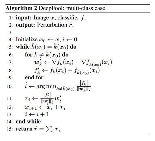
-
如上,对抗样本已经生成,存储在变量 adver_example_by_FOOL 中。
-
其中 adver_target,clean_example,clean_target,都是为了后面的可视化作准备。
2.3 测试鲁棒性
- 我们希望生成的对抗样本能使得靶模型有很低的准确率,即攻击效果好
import torch.utils.data as Data
def adver_attack_vgg(model,adver_example,target,name):
  adver_dataset = Data.TensorDataset(adver_example, target)
  loader = Data.DataLoader(
    dataset=adver_dataset,      # 数据,封装进Data.TensorDataset()类的数据
    batch_size=batch_size      # 每块的大小
    )
  correct_num = torch.tensor(0).to(device)
  for j,(data,target) in tqdm(enumerate(loader)):
    data = data.to(device)
    target = target.to(device)
    pred = model.forward(data).max(1)[1]
    num = torch.sum(pred==target)
    correct_num = correct_num + num
  print (correct_num)
  print ('\n{} correct rate is {}'.format(name,correct_num/adver_nums))

adver_attack_vgg(simple_model,adver_example_by_FOOL,clean_target,'simple model')
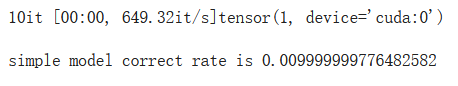
Output:
- 可以看出,deepfool的攻击效果是非常好的,模型分类准确度只达到了一个百分点。
2.4 可视化展示
def plot_clean_and_adver(adver_example,adver_target,clean_example,clean_target):
  n_cols = 5
  n_rows = 5
  cnt = 1
  cnt1 = 1
  plt.figure(figsize=(n_cols*4,n_rows*2))
  for i in range(n_cols):
    for j in range(n_rows):
      plt.subplot(n_cols,n_rows*2,cnt1)
      plt.xticks([])
      plt.yticks([])
      plt.title("{} -> {}".format(clean_target[cnt], adver_target[cnt]))
      plt.imshow(clean_example[cnt].reshape(28,28).to('cpu').detach().numpy(),cmap='gray')
      plt.subplot(n_cols,n_rows*2,cnt1+1)
      plt.xticks([])
      plt.yticks([])
      # plt.title("{} -> {}".format(clean_target[cnt], adver_target[cnt]))
      plt.imshow(adver_example[cnt].reshape(28,28).to('cpu').detach().numpy(),cmap='gray')
      cnt = cnt + 1
      cnt1 = cnt1 + 2
  plt.show()

plot_clean_and_adver(adver_example_by_FOOL,adver_target,clean_example,clean_target)
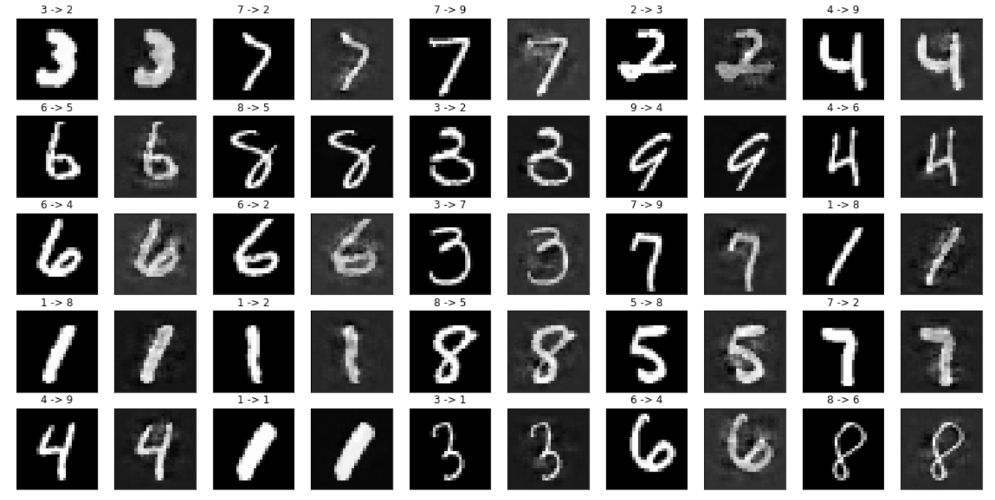
Output:
- 效果多好,你放大了看。左边是干净样本,右边是对抗样本,放在一起好对比效果。
附录
代码地址:
https://colab.research.google.com/drive/1g9i75kwQbw5vJbAjrZ87NA0P_wb7KXfw?usp=sharing


 1万+
1万+


 被折叠的 条评论
为什么被折叠?
被折叠的 条评论
为什么被折叠?
 到【灌水乐园】发言


