


4.3 自动梯度计算
虽然我们能够通过模块化的方式比较好地对神经网络进行组装,但是每个模块的梯度计算过程仍然十分繁琐且容易出错。在深度学习框架中,已经封装了自动梯度计算的功能,我们只需要聚焦模型架构,不再需要耗费精力进行计算梯度。
飞桨提供了paddle.nn.Layer类,来方便快速的实现自己的层和模型。模型和层都可以基于paddle.nn.Layer扩充实现,模型只是一种特殊的层。
继承了paddle.nn.Layer类的算子中,可以在内部直接调用其它继承paddle.nn.Layer类的算子,飞桨框架会自动识别算子中内嵌的paddle.nn.Layer类算子,并自动计算它们的梯度,并在优化时更新它们的参数。
4.3.1 利用预定义算子重新实现前馈神经网络
class Model_MLP_L2_V4(torch.nn.Module):
    def __init__(self, input_size, hidden_size, output_size):
        super(Model_MLP_L2_V4, self).__init__()
        self.fc1 = nn.Linear(input_size, hidden_size)
        w=torch.normal(0,0.1,size=(hidden_size,input_size),requires_grad=True)
        self.fc1.weight = nn.Parameter(w)

        self.fc2 = nn.Linear(hidden_size, output_size)
        w = torch.normal(0, 0.1, size=(output_size, hidden_size), requires_grad=True)
        self.fc2.weight = nn.Parameter(w)

        # 使用'torch.nn.functional.sigmoid'定义 Logistic 激活函数
        self.act_fn = torch.sigmoid

    # 前向计算
    def forward(self, inputs):
        z1 = self.fc1(inputs.to(torch.float32))
        a1 = self.act_fn(z1)
        z2 = self.fc2(a1)
        a2 = self.act_fn(z2)
        return a2
4.3.2 完善Runner类
class RunnerV2_2(object):
    def __init__(self, model, optimizer, metric, loss_fn, **kwargs):
        self.model = model
        self.optimizer = optimizer
        self.loss_fn = loss_fn
        self.metric = metric

        # 记录训练过程中的评估指标变化情况
        self.train_scores = []
        self.dev_scores = []

        # 记录训练过程中的评价指标变化情况
        self.train_loss = []
        self.dev_loss = []

    def train(self, train_set, dev_set, **kwargs):
        # 将模型切换为训练模式
        self.model.train()

        # 传入训练轮数,如果没有传入值则默认为0
        num_epochs = kwargs.get("num_epochs", 0)
        # 传入log打印频率,如果没有传入值则默认为100
        log_epochs = kwargs.get("log_epochs", 100)
        # 传入模型保存路径,如果没有传入值则默认为"best_model.pdparams"
        save_path = kwargs.get("save_path", "best_model.pdparams")

        # log打印函数,如果没有传入则默认为"None"
        custom_print_log = kwargs.get("custom_print_log", None)

        # 记录全局最优指标
        best_score = 0
        # 进行num_epochs轮训练
        for epoch in range(num_epochs):
            X, y = train_set

            # 获取模型预测
            logits = self.model(X.to(torch.float32))
            # 计算交叉熵损失
            trn_loss = self.loss_fn(logits, y)
            self.train_loss.append(trn_loss.item())
            # 计算评估指标
            trn_score = self.metric(logits, y).item()
            self.train_scores.append(trn_score)

            # 自动计算参数梯度
            trn_loss.backward()
            if custom_print_log is not None:
                # 打印每一层的梯度
                custom_print_log(self)

            # 参数更新
            self.optimizer.step()
            # 清空梯度
            self.optimizer.zero_grad()   # reset gradient

            dev_score, dev_loss = self.evaluate(dev_set)
            # 如果当前指标为最优指标,保存该模型
            if dev_score > best_score:
                self.save_model(save_path)
                print(f"[Evaluate] best accuracy performence has been updated: {best_score:.5f} --> {dev_score:.5f}")
                best_score = dev_score

            if log_epochs and epoch % log_epochs == 0:
                print(f"[Train] epoch: {epoch}/{num_epochs}, loss: {trn_loss.item()}")
    @torch.no_grad()
    def evaluate(self, data_set):
        # 将模型切换为评估模式
        self.model.eval()

        X, y = data_set
        # 计算模型输出
        logits = self.model(X)
        # 计算损失函数
        loss = self.loss_fn(logits, y).item()
        self.dev_loss.append(loss)
        # 计算评估指标
        score = self.metric(logits, y).item()
        self.dev_scores.append(score)
        return score, loss

    # 模型测试阶段,使用'torch.no_grad()'控制不计算和存储梯度
    @torch.no_grad()
    def predict(self, X):
        # 将模型切换为评估模式
        self.model.eval()
        return self.model(X)

    # 使用'model.state_dict()'获取模型参数,并进行保存
    def save_model(self, saved_path):
        torch.save(self.model.state_dict(), saved_path)

    # 使用'model.set_state_dict'加载模型参数
    def load_model(self, model_path):
        state_dict = torch.load(model_path)
        self.model.load_state_dict(state_dict)
4.3.3 模型训练
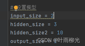
# 设置模型
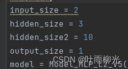
input_size = 2
hidden_size = 5
output_size = 1
model = Model_MLP_L2_V4(input_size=input_size, hidden_size=hidden_size, output_size=output_size)
# 设置损失函数
loss_fn = F.binary_cross_entropy
# 设置优化器
learning_rate = 0.2 #5e-2
optimizer = torch.optim.SGD(model.parameters(),lr=learning_rate)
# 设置评价指标
metric = accuracy
# 其他参数
epoch = 2000
saved_path = 'best_model.pdparams'
# 实例化RunnerV2类,并传入训练配置
runner = RunnerV2_2(model, optimizer, metric, loss_fn)
runner.train([X_train, y_train], [X_dev, y_dev], num_epochs = epoch, log_epochs=50, save_path="best_model.pdparams")
plot(runner, 'fw-acc.pdf')
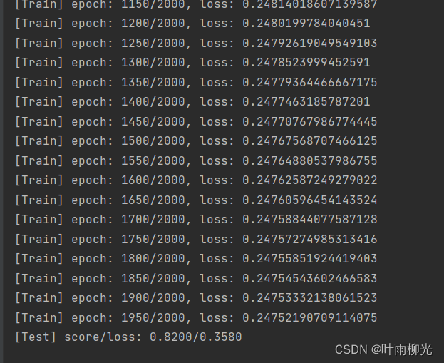
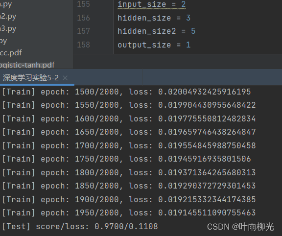
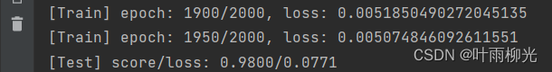
4.3.4 性能评价
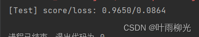
#模型评价
runner.load_model("best_model.pdparams")
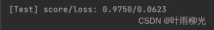
score, loss = runner.evaluate([X_test, y_test])
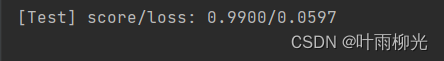
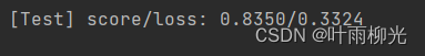
print("[Test] score/loss: {:.4f}/{:.4f}".format(score, loss))
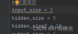
# 设置模型
input_size = 2
hidden_size = 5
hidden_size2 = 3
output_size = 1
model = Model_MLP_L2_V5(input_size=input_size, hidden_size=hidden_size,hidden_size2=hidden_size2, output_size=output_size)
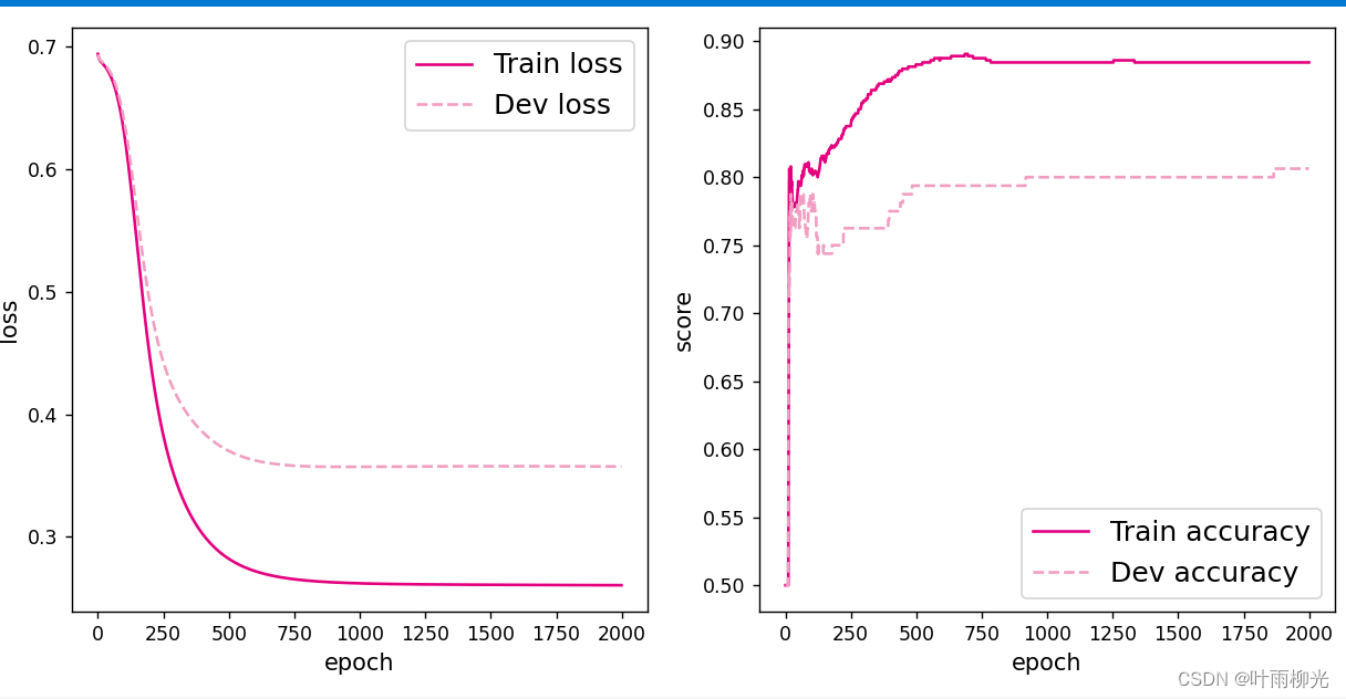
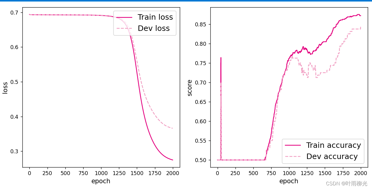
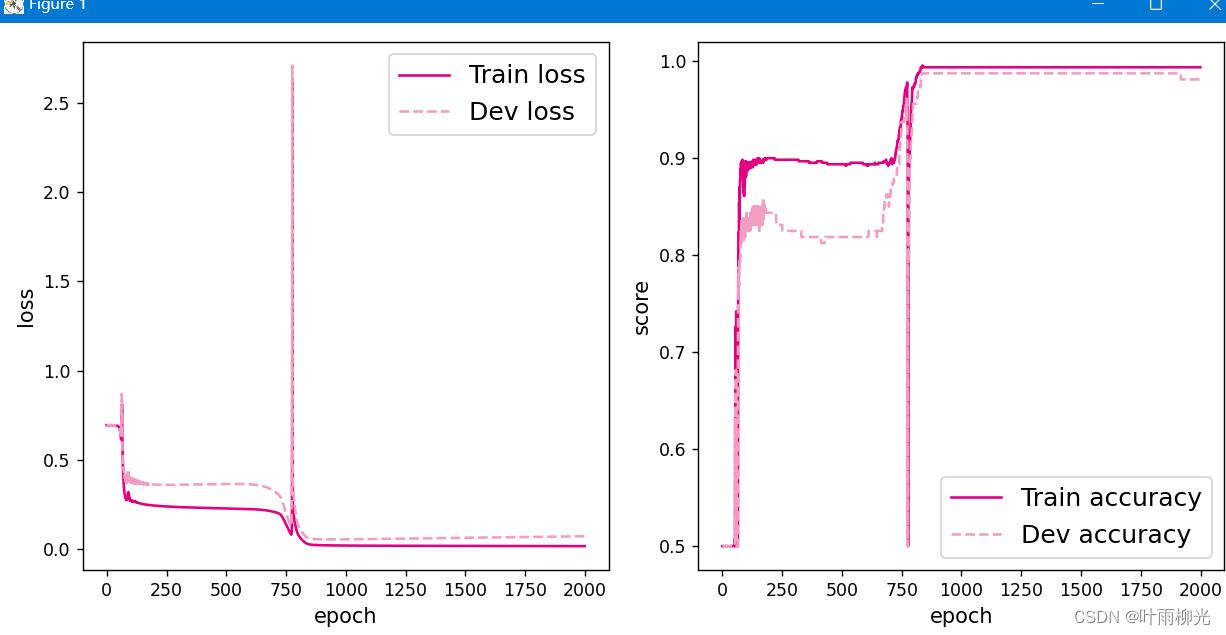
将训练过程中训练集与验证集的准确率变化情况进行可视化。
# 可视化观察训练集与验证集的指标变化情况
def plot(runner, fig_name):
    plt.figure(figsize=(10,5))
    epochs = [i for i in range(len(runner.train_scores))]

    plt.subplot(1,2,1)
    plt.plot(epochs, runner.train_loss, color='#e4007f', label="Train loss")
    plt.plot(epochs, runner.dev_loss, color='#f19ec2', linestyle='--', label="Dev loss")
    # 绘制坐标轴和图例
    plt.ylabel("loss", fontsize='large')
    plt.xlabel("epoch", fontsize='large')
    plt.legend(loc='upper right', fontsize='x-large')

    plt.subplot(1,2,2)
    plt.plot(epochs, runner.train_scores, color='#e4007f', label="Train accuracy")
    plt.plot(epochs, runner.dev_scores, color='#f19ec2', linestyle='--', label="Dev accuracy")
    # 绘制坐标轴和图例
    plt.ylabel("score", fontsize='large')
    plt.xlabel("epoch", fontsize='large')
    plt.legend(loc='lower right', fontsize='x-large')

    plt.savefig(fig_name)
    plt.show()

plot(runner, 'fw-acc.pdf')
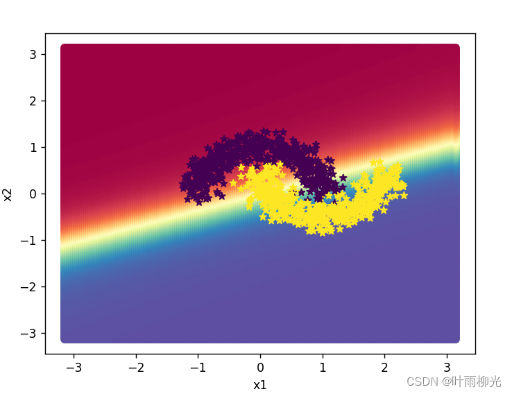
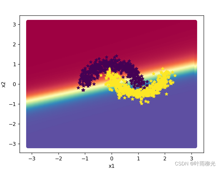
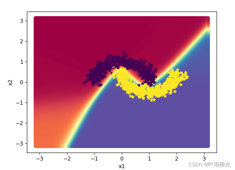
使用pytorch的预定义算子来重新实现二分类任务。
import math
import matplotlib.pyplot as plt
# 均匀生成40000个数据点
x1, x2 = torch.meshgrid(torch.linspace(-math.pi, math.pi, 200), torch.linspace(-math.pi, math.pi, 200))

x = torch.stack([torch.flatten(x1), torch.flatten(x2)], axis=1)

# 预测对应类别
y = runner.predict(x)
# y = torch.squeeze(torch.as_tensor(torch.can_cast((y>=0.5).dtype,torch.float32)))

# 绘制类别区域
plt.ylabel('x2')
plt.xlabel('x1')
plt.scatter(x[:,0].tolist(), x[:,1].tolist(), c=y.tolist(), cmap=plt.cm.Spectral)

plt.scatter(X_train[:, 0].tolist(), X_train[:, 1].tolist(), marker='*', c=torch.squeeze(y_train,axis=-1).tolist())
plt.scatter(X_dev[:, 0].tolist(), X_dev[:, 1].tolist(), marker='*', c=torch.squeeze(y_dev,axis=-1).tolist())
plt.scatter(X_test[:, 0].tolist(), X_test[:, 1].tolist(), marker='*', c=torch.squeeze(y_test,axis=-1).tolist())

plt.show()
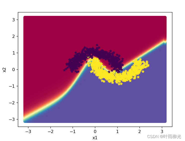
增加一个3个神经元的隐藏层,再次实现二分类,并与1做对比。
class Model_MLP_L2_V5(torch.nn.Module):
    def __init__(self, input_size, hidden_size, hidden_size2, output_size):
        super(Model_MLP_L2_V5, self).__init__()
        self.fc1 = nn.Linear(input_size, hidden_size)
        w1=torch.normal(0,0.1,size=(hidden_size,input_size),requires_grad=True)
        self.fc1.weight = nn.Parameter(w1)

        self.fc2 = nn.Linear(hidden_size, hidden_size2)
        w2 = torch.normal(0, 0.1, size=(hidden_size2, hidden_size), requires_grad=True)
        self.fc2.weight = nn.Parameter(w2)

        self.fc3 = nn.Linear(hidden_size2, output_size)
        w3 = torch.normal(0, 0.1, size=(output_size, hidden_size2), requires_grad=True)
        self.fc3.weight = nn.Parameter(w3)

        # 使用'torch.nn.functional.sigmoid'定义 Logistic 激活函数
        self.act_fn = torch.sigmoid
 # 前向计算
    def forward(self, inputs):
        z1 = self.fc1(inputs.to(torch.float32))
        a1 = self.act_fn(z1)
        z2 = self.fc2(a1)
        a2 = self.act_fn(z2)
        z3 = self.fc3(a2)
        a3 = self.act_fn(z3)
        return a3
input_size = 2
hidden_size = 5
hidden_size2 = 3
output_size = 1
model = Model_MLP_L2_V5(input_size=input_size, hidden_size=hidden_size,hidden_size2=hidden_size2, output_size=output_size)
在lr=0.2的情况下:
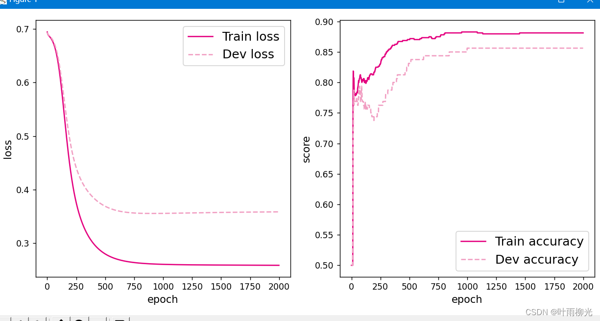
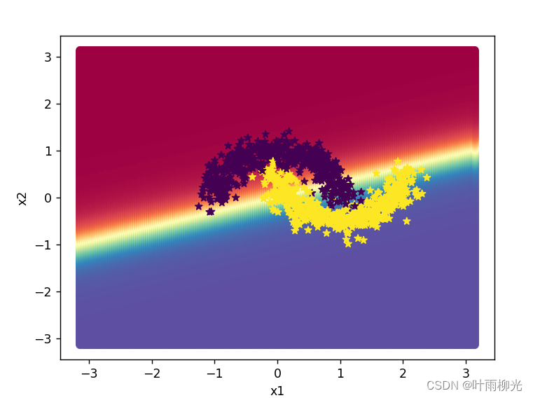
lr=5:
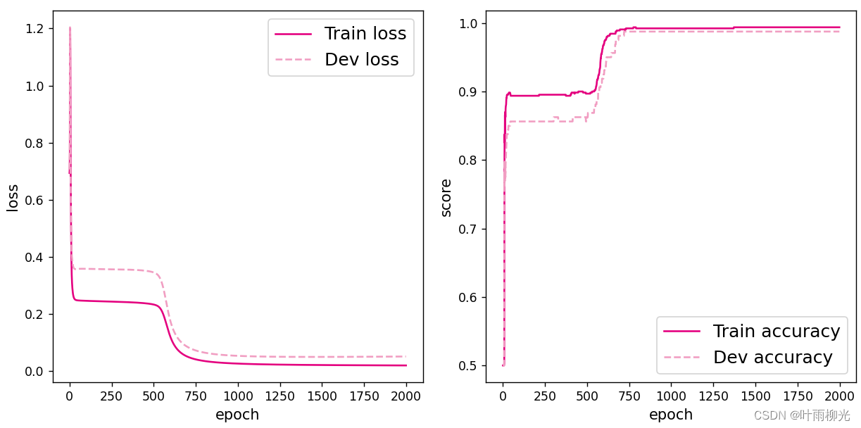
这里试了好多次没有截图,大概就是lr=5最优,就截图了这两种。
自定义隐藏层层数和每个隐藏层中的神经元个数,尝试找到最优超参数完成二分类。可以适当修改数据集,便于探索超参数。
2个隐藏层,lr=5:
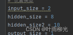
改2层神经元个数


二层最优大概为10
改一层个数
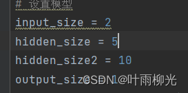


一层大概为3-5
一层隐藏层


3-5较好
【思考题】
自定义梯度计算和自动梯度计算:
从计算性能、计算结果等多方面比较,谈谈自己的看法。
自动:
自定义:


答:自定义梯度计算的准确率要大于自动梯度计算的准确率
4.4 优化问题
4.4.1 参数初始化
实现一个神经网络前,需要先初始化模型参数。
如果对每一层的权重和偏置都用0初始化,那么通过第一遍前向计算,所有隐藏层神经元的激活值都相同;在反向传播时,所有权重的更新也都相同,这样会导致隐藏层神经元没有差异性,出现对称权重现象。
# import torch
import torch.nn as nn
import torch.nn.functional as F
# 定义多层前馈神经网络
class Model_MLP_L2_V4(torch.nn.Module):
    def __init__(self, input_size, hidden_size,output_size):
        super(Model_MLP_L2_V4, self).__init__()
        self.fc1 = nn.Linear(input_size, hidden_size)
        # w1=torch.normal(0,0.1,size=(hidden_size,input_size),requires_grad=True)
        # self.fc1.weight = nn.Parameter(w1)
        self.fc1.weight=nn.init.constant_(self.fc1.weight,val=0.0)
        # self.fc1.bias = nn.init.constant_(self.fc1.bias, val=1.0)
        self.fc1.bias = nn.init.constant_(self.fc1.bias, val=0.0)
        self.fc2 = nn.Linear(hidden_size, output_size)
        # w2 = torch.normal(0, 0.1, size=(output_size, hidden_size), requires_grad=True)
        # self.fc2.weight = nn.Parameter(w2)
        self.fc2.weight = nn.init.constant_(self.fc2.weight, val=0.0)
        self.fc2.bias = nn.init.constant_(self.fc2.bias, val=0.0)
        # 使用'torch.nn.functional.sigmoid'定义 Logistic 激活函数
        self.act_fn = torch.sigmoid

    # 前向计算
    def forward(self, inputs):
        z1 = self.fc1(inputs.to(torch.float32))
        a1 = self.act_fn(z1)
        z2 = self.fc2(a1)
        a2 = self.act_fn(z2)
        return a2
def print_weights(runner):
    print('The weights of the Layers:')

    for item in runner.model.sublayers():
        print(item.full_name())
        for param in item.parameters():
            print(param.numpy())
利用Runner类训练模型:
# 设置模型
input_size = 2
hidden_size = 5
output_size = 1
model = Model_MLP_L2_V4(input_size=input_size, hidden_size=hidden_size, output_size=output_size)

# 设置损失函数
loss_fn = F.binary_cross_entropy

# 设置优化器
learning_rate = 0.2#5e-2
optimizer = torch.optim.SGD(model.parameters(),lr=learning_rate)

# 设置评价指标
metric = accuracy

# 其他参数
epoch = 2000
saved_path = 'best_model.pdparams'

# 实例化RunnerV2类,并传入训练配置
runner = RunnerV2_2(model, optimizer, metric, loss_fn)

runner.train([X_train, y_train], [X_dev, y_dev], num_epochs = epoch, log_epochs=50, save_path="best_model.pdparams")
for _,param in enumerate(runner.model.named_parameters()):
  print(param)
  print('---------------------------------')
 plot(runner, "fw-zero.pdf")
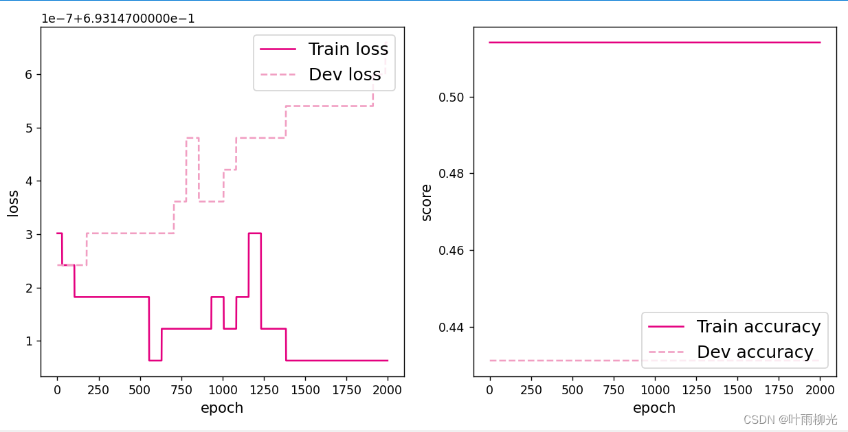
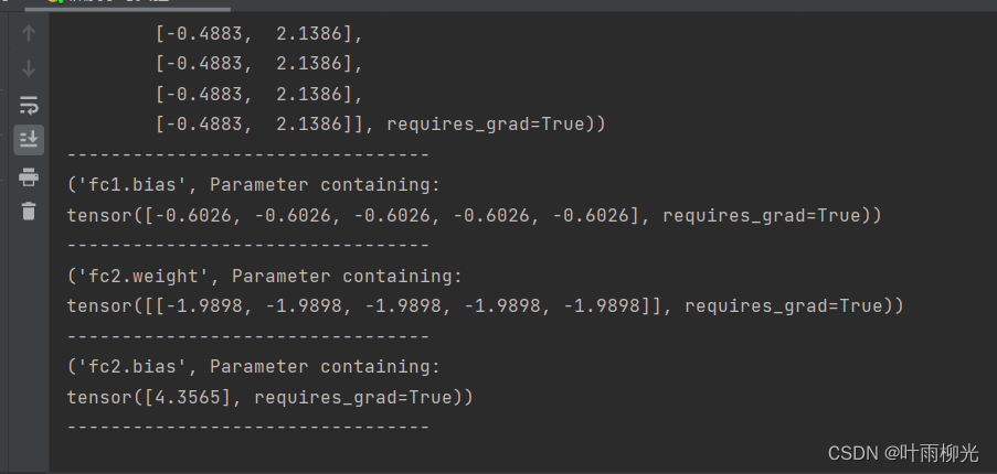
从输出结果看,二分类准确率为50%左右,说明模型没有学到任何内容。训练和验证loss几乎没有怎么下降。
为了避免对称权重现象,可以使用高斯分布或均匀分布初始化神经网络的参数。
4.4.2 梯度消失问题
在神经网络的构建过程中,随着网络层数的增加,理论上网络的拟合能力也应该是越来越好的。但是随着网络变深,参数学习更加困难,容易出现梯度消失问题。
由于Sigmoid型函数的饱和性,饱和区的导数更接近于0,误差经过每一层传递都会不断衰减。当网络层数很深时,梯度就会不停衰减,甚至消失,使得整个网络很难训练,这就是所谓的梯度消失问题。
在深度神经网络中,减轻梯度消失问题的方法有很多种,一种简单有效的方式就是使用导数比较大的激活函数,如:ReLU。
下面通过一个简单的实验观察前馈神经网络的梯度消失现象和改进方法。
4.4.2.1 模型构建
# 定义多层前馈神经网络
class Model_MLP_L5(torch.nn.Module):
    def __init__(self, input_size, output_size, act='relu'):
        super(Model_MLP_L5, self).__init__()
        self.fc1 = torch.nn.Linear(input_size, 3)
        w_ = torch.normal(0, 0.01, size=(3, input_size), requires_grad=True)
        self.fc1.weight = nn.Parameter(w_)
        self.fc1.bias = nn.init.constant_(self.fc1.bias, val=1.0)
        w= torch.normal(0, 0.01, size=(3, 3), requires_grad=True)

        self.fc2 = torch.nn.Linear(3, 3)
        self.fc2.weight = nn.Parameter(w)
        self.fc2.bias = nn.init.constant_(self.fc2.bias, val=1.0)
        self.fc3 = torch.nn.Linear(3, 3)
        self.fc3.weight = nn.Parameter(w)
        self.fc3.bias = nn.init.constant_(self.fc3.bias, val=1.0)
        self.fc4 = torch.nn.Linear(3, 3)
        self.fc4.weight = nn.Parameter(w)
        self.fc4.bias = nn.init.constant_(self.fc4.bias, val=1.0)
        self.fc5 = torch.nn.Linear(3, output_size)
        w1 = torch.normal(0, 0.01, size=(output_size, 3), requires_grad=True)
        self.fc5.weight = nn.Parameter(w1)
        self.fc5.bias = nn.init.constant_(self.fc5.bias, val=1.0)
        # 定义网络使用的激活函数
        if act == 'sigmoid':
            self.act = F.sigmoid
        elif act == 'relu':
            self.act = F.relu
        elif act == 'lrelu':
            self.act = F.leaky_relu
        else:
            raise ValueError("Please enter sigmoid relu or lrelu!")


    def forward(self, inputs):
        outputs = self.fc1(inputs.to(torch.float32))
        outputs = self.act(outputs)
        outputs = self.fc2(outputs)
        outputs = self.act(outputs)
        outputs = self.fc3(outputs)
        outputs = self.act(outputs)
        outputs = self.fc4(outputs)
        outputs = self.act(outputs)
        outputs = self.fc5(outputs)
        outputs = F.sigmoid(outputs)
        return outputs
4.4.2.2 使用Sigmoid型函数进行训练
# 学习率大小
lr = 0.01
# 定义网络,激活函数使用sigmoid
model = Model_MLP_L5(input_size=2, output_size=1, act='sigmoid')
# 定义优化器
optimizer = torch.optim.SGD(model.parameters(),lr=lr)
# 定义损失函数,使用交叉熵损失函数
loss_fn = F.binary_cross_entropy
# 定义评价指标
metric = accuracy
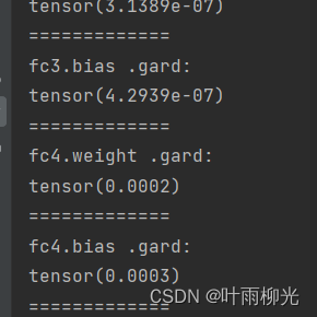
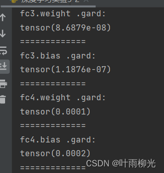
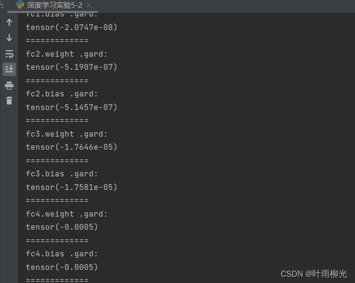
def print_grads(runner):
# 打印每一层的权重的模
print('The gradient of the Layers:')
for item in runner.model.named_parameters():
if len(item[1])==3:
print(item[0],".gard:")
print(torch.mean(item[1].grad))
print("=============")
# 指定梯度打印函数
custom_print_log = print_grads
# 实例化Runner类
runner = RunnerV2_2(model, optimizer, metric, loss_fn)
# 启动训练
runner.train([X_train, y_train], [X_dev, y_dev],
num_epochs=1, log_epochs=None,
save_path="best_model.pdparams",
custom_print_log=custom_print_log)
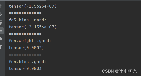
观察实验结果可以发现,梯度经过每一个神经层的传递都会不断衰减,最终传递到第一个神经层时,梯度几乎完全消失。
4.4.2.3 使用ReLU函数进行模型训练
torch.manual_seed(102)
# 学习率大小
lr = 0.01

# 定义网络,激活函数使用sigmoid
model = Model_MLP_L5(input_size=2, output_size=1, act='sigmoid')

# 定义优化器
optimizer = torch.optim.SGD(model.parameters(), lr)

# 定义损失函数,使用交叉熵损失函数
loss_fn = F.binary_cross_entropy

# 定义评价指标
metric = accuracy

# 指定梯度打印函数
custom_print_log = print_grads
# 实例化Runner类
runner = RunnerV2_2(model, optimizer, metric, loss_fn)
# 启动训练
runner.train([X_train, y_train], [X_dev, y_dev],
             num_epochs=1, log_epochs=None,
             save_path="best_model.pdparams",
             custom_print_log=custom_print_log)
4.4.3 死亡ReLU问题
ReLU激活函数可以一定程度上改善梯度消失问题,但是ReLU函数在某些情况下容易出现死亡 ReLU问题,使得网络难以训练。这是由于当x<0时,ReLU函数的输出恒为0。在训练过程中,如果参数在一次不恰当的更新后,某个ReLU神经元在所有训练数据上都不能被激活(即输出为0),那么这个神经元自身参数的梯度永远都会是0,在以后的训练过程中永远都不能被激活。而一种简单有效的优化方式就是将激活函数更换为Leaky ReLU、ELU等ReLU的变种。
4.4.3.1 使用ReLU进行模型训练
# 定义多层前馈神经网络
class Model_MLP_L5(torch.nn.Module):
    def __init__(self, input_size, output_size, act='relu'):
        super(Model_MLP_L5, self).__init__()
        self.fc1 = torch.nn.Linear(input_size, 3)
        w_ = torch.normal(0, 0.01, size=(3, input_size), requires_grad=True)
        self.fc1.weight = nn.Parameter(w_)
        # self.fc1.bias = nn.init.constant_(self.fc1.bias, val=1.0)
        self.fc1.bias = nn.init.constant_(self.fc1.bias, val=-8.0)
        w= torch.normal(0, 0.01, size=(3, 3), requires_grad=True)

        self.fc2 = torch.nn.Linear(3, 3)
        self.fc2.weight = nn.Parameter(w)
        # self.fc2.bias = nn.init.constant_(self.fc2.bias, val=1.0)
        self.fc1.bias = nn.init.constant_(self.fc1.bias, val=-8.0)
        self.fc3 = torch.nn.Linear(3, 3)
        self.fc3.weight = nn.Parameter(w)
        # self.fc3.bias = nn.init.constant_(self.fc2.bias, val=1.0)
        self.fc3.bias = nn.init.constant_(self.fc3.bias, val=-8.0)
        self.fc4 = torch.nn.Linear(3, 3)
        self.fc4.weight = nn.Parameter(w)
        # self.fc4.bias = nn.init.constant_(self.fc2.bias, val=1.0)
        self.fc4.bias = nn.init.constant_(self.fc4.bias, val=-8.0)
        self.fc5 = torch.nn.Linear(3, output_size)
        w1 = torch.normal(0, 0.01, size=(output_size, 3), requires_grad=True)
        self.fc5.weight = nn.Parameter(w1)
        # self.fc5.bias = nn.init.constant_(self.fc2.bias, val=1.0)
        self.fc5.bias = nn.init.constant_(self.fc5.bias, val=-8.0)
        # 定义网络使用的激活函数
        if act == 'sigmoid':
            self.act = F.sigmoid
        elif act == 'relu':
            self.act = F.relu
        elif act == 'lrelu':
            self.act = F.leaky_relu
        else:
            raise ValueError("Please enter sigmoid relu or lrelu!")


    def forward(self, inputs):
        outputs = self.fc1(inputs.to(torch.float32))
        outputs = self.act(outputs)
        outputs = self.fc2(outputs)
        outputs = self.act(outputs)
        outputs = self.fc3(outputs)
        outputs = self.act(outputs)
        outputs = self.fc4(outputs)
        outputs = self.act(outputs)
        outputs = self.fc5(outputs)
        outputs = F.sigmoid(outputs)
        return outputs
从输出结果可以发现,使用 ReLU 作为激活函数,当满足条件时,会发生死亡ReLU问题,网络训练过程中 ReLU 神经元的梯度始终为0,参数无法更新。针对死亡ReLU问题,一种简单有效的优化方式就是将激活函数更换为Leaky ReLU、ELU等ReLU 的变种。接下来,观察将激活函数更换为 Leaky ReLU时的梯度情况。
4.4.3.2 使用Leaky ReLU进行模型训练
# 定义网络,激活函数使用sigmoid
model = Model_MLP_L5(input_size=2, output_size=1, act='lrelu')


# 实例化Runner类
runner = RunnerV2_2(model, optimizer, metric, loss_fn)

# 启动训练
runner.train([X_train, y_train], [X_dev, y_dev],
            num_epochs=1, log_epochps=None,
            save_path="best_model.pdparams",
            custom_print_log=custom_print_log)
总结
有些问题没搞懂,梯度哪里不知道为什么不为0,之后在看看。


 488
488


 被折叠的 条评论
为什么被折叠?
被折叠的 条评论
为什么被折叠?
 到【灌水乐园】发言


