逻辑斯谛回归与最大熵模型的原理实现

最新推荐文章于 2024-07-01 14:40:42 发布

铃之

最新推荐文章于 2024-07-01 14:40:42 发布

阅读量351

点赞数 5

分类专栏：机器学习文章标签：回归数据挖掘人工智能分类最大熵模型逻辑回归机器学习

本文链接：https://blog.csdn.net/m0_56676945/article/details/139685350

版权

机器学习专栏收录该内容

20 篇文章 3 订阅

订阅专栏

逻辑斯谛回归(LR)是经典的分类方法

1．逻辑斯谛回归模型是由以下条件概率分布表示的分类模型。逻辑斯谛回归模型可以用于二类或多类分类。

$x)=\frac{\exp \left(w_{k} \cdot x\right)}{1+\sum_{k=1}^{K-1} \exp \left(w_{k} \cdot x\right)}, \quad k=1,2, \cdots, K-1$

$x)=\frac{1}{1+\sum_{k=1}^{K-1} \exp \left(w_{k} \cdot x\right)}$
这里， $x$ 为输入特征， $w$ 为特征的权值。

逻辑斯谛回归模型源自逻辑斯谛分布，其分布函数 $F (x)$ 是 $S$ 形函数。逻辑斯谛回归模型是由输入的线性函数表示的输出的对数几率模型。

2．最大熵模型是由以下条件概率分布表示的分类模型。最大熵模型也可以用于二类或多类分类。

$P_{w}(y | x)=\frac{1}{Z_{w}(x)} \exp \left(\sum_{i=1}^{n} w_{i} f_{i}(x, y)\right)$
$Z_{w}(x)=\sum_{y} \exp \left(\sum_{i=1}^{n} w_{i} f_{i}(x, y)\right)$

其中， $Z_w(x)$ 是规范化因子， $f_i$ 为特征函数， $w_i$ 为特征的权值。

3．最大熵模型可以由最大熵原理推导得出。最大熵原理是概率模型学习或估计的一个准则。最大熵原理认为在所有可能的概率模型（分布）的集合中，熵最大的模型是最好的模型。

最大熵原理应用到分类模型的学习中，有以下约束最优化问题：

$\min -H(P)=\sum_{x, y} \tilde{P}(x) P(y | x) \log P(y | x)$

$\quad P\left(f_{i}\right)-\tilde{P}\left(f_{i}\right)=0, \quad i=1,2, \cdots, n$

$\sum_{y} P(y | x)=1$

求解此最优化问题的对偶问题得到最大熵模型。

4．逻辑斯谛回归模型与最大熵模型都属于对数线性模型。

5．逻辑斯谛回归模型及最大熵模型学习一般采用极大似然估计，或正则化的极大似然估计。逻辑斯谛回归模型及最大熵模型学习可以形式化为无约束最优化问题。求解该最优化问题的算法有改进的迭代尺度法、梯度下降法、拟牛顿法。

逻辑斯谛回归

1. 模型和假设函数

逻辑回归模型的假设函数（或预测函数）是：
$h_\theta(x) = \sigma(\theta^T x) = \frac{1}{1 + e^{-\theta^T x}}$

其中：

$\theta$ 是参数向量。
$x$ 是特征向量。
$\sigma(z)$ 是 $s i g m o i d$ 函数。

2. 损失函数

逻辑回归通常使用对数似然损失函数，其形式为：
$L(\theta) = -\frac{1}{m} \sum_{i=1}^{m} \left[ y^{(i)} \log(h_\theta(x^{(i)})) + (1 - y^{(i)}) \log(1 - h_\theta(x^{(i)})) \right]$

其中：

$m$ 是训练样本的数量。
$y^{(i)}$ 是第 $i$ 个训练样本的真实标签。
$h_\theta(x^{(i)})$ 是第 $i$ 个训练样本的预测值。

3. 梯度下降算法

为了最小化损失函数，需要计算损失函数关于参数的梯度，并更新参数。梯度下降的更新规则如下：

计算梯度：损失函数关于参数 $\theta$ 的梯度为：
$\frac{\partial L(\theta)}{\partial \theta_j} = \frac{1}{m} \sum_{i=1}^{m} \left( h_\theta(x^{(i)}) - y^{(i)}) \right) x_j^{(i)}$
参数更新：使用梯度下降法更新参数：
$\theta_j := \theta_j - \alpha \frac{\partial L(\theta)}{\partial \theta_j}$

其中：

$\alpha$ 是学习率，控制每次更新的步长。
$x_j^{(i)}$ 是第 $i$ 个训练样本中第 $j$ 个特征的值。

4. 具体步骤

假设有一个训练集 ${(x^{(i)}, y^{(i)})\}_{i=1}^{m}$ ，逻辑回归的梯度下降算法的步骤如下：

初始化参数：将参数 $\theta$ 初始化为零或小随机值。
重复直到收敛：
- 计算每个训练样本的预测值：
  $h_\theta(x^{(i)}) = \frac{1}{1 + e^{-\theta^T x^{(i)}}}$
- 计算梯度：
  $\frac{\partial L(\theta)}{\partial \theta_j} = \frac{1}{m} \sum_{i=1}^{m} \left( h_\theta(x^{(i)}) - y^{(i)} \right) x_j^{(i)}$
- 更新参数：
  $\theta_j := \theta_j - \alpha \frac{\partial L(\theta)}{\partial \theta_j}$

import numpy as np
import pandas as pd
import matplotlib.pyplot as plt
from sklearn.datasets import load_iris
from sklearn.model_selection import train_test_split
from matplotlib_inline import backend_inline

backend_inline.set_matplotlib_formats('svg')

# 获取数据
def create_data():
    iris = load_iris()
    df = pd.DataFrame(iris.data, columns=iris.feature_names)
    df['label'] = iris.target
    df.columns = [
        "sepal length", "sepal width", "petal length", "petal width", "label"
    ]
    data = np.array(df.iloc[:100, [0, 1, -1]])
    # print(data)
    return data[:, :2], data[:, -1]


X, y = create_data()
X_train, X_test, y_train, y_test = train_test_split(X,
                                                    y,
                                                    test_size=0.3,
                                                    random_state=42)

class LogisticReressionClassifier:
    def __init__(self, num_iterations=200, learning_rate=0.01):
        self.num_iterations = num_iterations
        self.learning_rate = learning_rate

    # sigmoid 函数
    def sigmoid(self, z):
        return 1 / (1 + np.exp(-z))

    # X加一列1
    def data_matrix(self, X):
        data_mat = []
        for d in X:
            data_mat.append([1.0, *d])
        return np.array(data_mat)

    # 计算损失函数的梯度
    def compute_gradient(self, X, y, theta):
        m = len(y)
        h = self.sigmoid(np.dot(X, theta))
        gradient = (1 / m) * np.transpose(X).dot(h - y)  # 矩阵乘法自动包含了对所有样本进行求和运算
        return gradient

    # 梯度下降算法
    def fit(self, X, y):
        X_data = self.data_matrix(X)
        y = y.reshape(-1, 1)
        self.theta = np.zeros((len(X_data[0]), 1), dtype=np.float32)
        for _ in range(self.num_iterations):
            gradient = self.compute_gradient(X_data, y, self.theta)
            self.theta -= self.learning_rate * gradient
        print(self.theta)

    def score(self, X_test, y_test):
        right = 0
        X_test = self.data_matrix(X_test)
        y_test = y_test.reshape(-1, 1)
        for x, y in zip(X_test, y_test):
            result = np.dot(x, self.theta)
            if (result > 0 and y == 1) or (result < 0 and y == 0):
                right += 1
        return right / len(X_test)

lr_clf = LogisticReressionClassifier()
lr_clf.fit(X_train, y_train)

[[-0.03514242]
 [ 0.2566241 ]
 [-0.3842345 ]]

lr_clf.score(X_test, y_test)

0.8333333333333334

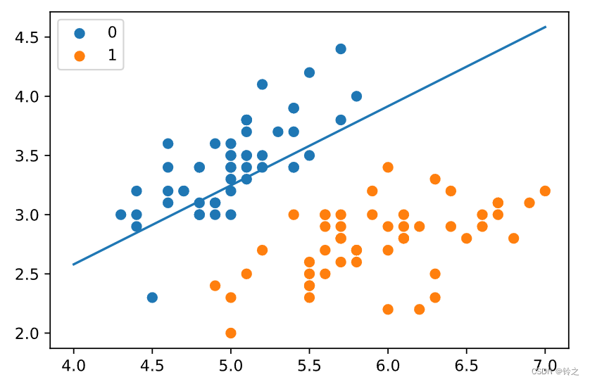
x1 = np.arange(4, 8)
x2 = -(lr_clf.theta[1] * x1 + lr_clf.theta[0]) / lr_clf.theta[2]
plt.plot(x1, x2)

#lr_clf.show_graph()
plt.scatter(X[:50, 0], X[:50, 1], label='0')
plt.scatter(X[50:, 0], X[50:, 1], label='1')
plt.legend()
plt.show()

在这里插入图片描述

使用sklearn实现：sklearn.linear_model.LogisticRegression

solver参数决定了我们对逻辑回归损失函数的优化方法，有四种算法可以选择，分别是：

a) liblinear：使用了开源的liblinear库实现，内部使用了坐标轴下降法来迭代优化损失函数。
b) lbfgs：拟牛顿法的一种，利用损失函数二阶导数矩阵即海森矩阵来迭代优化损失函数。
c) newton-cg：也是牛顿法家族的一种，利用损失函数二阶导数矩阵即海森矩阵来迭代优化损失函数。
d) sag：即随机平均梯度下降，是梯度下降法的变种，和普通梯度下降法的区别是每次迭代仅仅用一部分的样本来计算梯度，适合于样本数据多的时候。

from sklearn.linear_model import LogisticRegression

clf = LogisticRegression(max_iter=200)
clf.fit(X_train, y_train)
print(clf.score(X_test, y_test))
print(clf.coef_, clf.intercept_)

1.0
[[ 2.73483153 -2.58584717]] [-6.72555857]

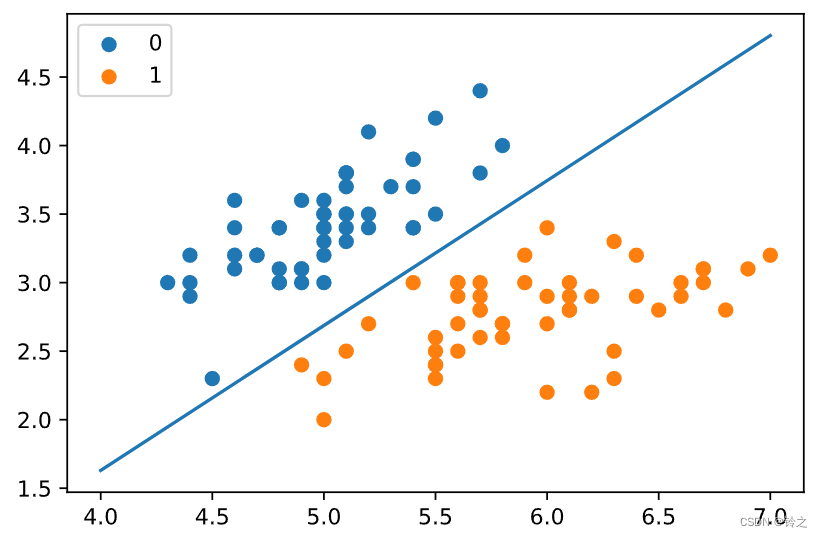
x1 = np.arange(4, 8)
x2 = -(clf.coef_[0][0] * x1 + clf.intercept_[0]) / clf.coef_[0][1]
plt.plot(x1, x2)

#lr_clf.show_graph()
plt.scatter(X[:50, 0], X[:50, 1], label='0')
plt.scatter(X[50:, 0], X[50:, 1], label='1')
plt.legend()
plt.show()

在这里插入图片描述

最大熵模型

最大熵模型 $（ M a x im u m E n t ro p y M o d e l ）$ 是一种用于分类和回归问题的概率模型，基于最大熵原理。最大熵原理提出，在所有符合约束条件的概率分布中，应选择熵最大的那个，因为它表示最不确定的、最没有偏见的分布。最大熵模型通常用于自然语言处理中的分类任务，如文本分类、词性标注等。

这段代码实现了一个用于多分类任务的最大熵模型，并使用改进的迭代尺度算法 $（ I m p ro v e d I t er a t i v e S c a l in g, II S ）$ 来训练模型参数。

import math
from copy import deepcopy


class MaxEntropy:
    def __init__(self, EPS=0.005):
        self._samples = []
        self._Y = set()  # 标签集合，相当去去重后的y
        self._numXY = {}  # key为(x,y)，value为出现次数
        self._N = 0  # 样本数
        self._Ep_ = []  # 样本分布的特征期望值
        self._xyID = {}  # key记录(x,y),value记录id号
        self._n = 0  # 特征键值(x,y)的个数
        self._C = 0  # 最大特征数
        self._IDxy = {}  # key为(x,y)，value为对应的id号
        self._w = []
        self._EPS = EPS  # 收敛条件
        self._lastw = []  # 上一次w参数值

    def loadData(self, dataset):
        self._samples = deepcopy(dataset)
        for items in self._samples:
            y = items[0]
            X = items[1:]
            self._Y.add(y)  # 集合中y若已存在则会自动忽略
            for x in X:
                if (x, y) in self._numXY:
                    self._numXY[(x, y)] += 1
                else:
                    self._numXY[(x, y)] = 1

        self._N = len(self._samples)
        self._n = len(self._numXY)
        self._C = max([len(sample) - 1 for sample in self._samples])
        self._w = [0] * self._n
        self._lastw = self._w[:]

        self._Ep_ = [0] * self._n
        for i, xy in enumerate(self._numXY):  # 计算特征函数fi关于经验分布的期望
            self._Ep_[i] = self._numXY[xy] / self._N
            self._xyID[xy] = i
            self._IDxy[i] = xy

    def _Zx(self, X):  # 计算每个Z(x)值
        zx = 0
        for y in self._Y:
            ss = 0
            for x in X:
                if (x, y) in self._numXY:
                    ss += self._w[self._xyID[(x, y)]]
            zx += math.exp(ss)
        return zx

    def _model_pyx(self, y, X):  # 计算每个P(y|x)
        zx = self._Zx(X)
        ss = 0
        for x in X:
            if (x, y) in self._numXY:
                ss += self._w[self._xyID[(x, y)]]
        pyx = math.exp(ss) / zx
        return pyx

    def _model_ep(self, index):  # 计算特征函数fi关于模型的期望
        x, y = self._IDxy[index]
        ep = 0
        for sample in self._samples:
            if x not in sample:
                continue
            pyx = self._model_pyx(y, sample)
            ep += pyx / self._N
        return ep

    def _convergence(self):  # 判断是否全部收敛
        for last, now in zip(self._lastw, self._w):
            if abs(last - now) >= self._EPS:
                return False
        return True

    def predict(self, X):  # 计算预测概率
        Z = self._Zx(X)
        result = {}
        for y in self._Y:
            ss = 0
            for x in X:
                if (x, y) in self._numXY:
                    ss += self._w[self._xyID[(x, y)]]
            pyx = math.exp(ss) / Z
            result[y] = pyx
        return result

    def train(self, maxiter=1000):  # 训练数据
        for loop in range(maxiter):  # 最大训练次数
            print("iter:%d" % loop)
            self._lastw = self._w[:]
            for i in range(self._n):
                ep = self._model_ep(i)  # 计算第i个特征的模型期望
                self._w[i] += math.log(self._Ep_[i] / ep) / self._C  # 更新参数
            print("w:", self._w)
            if self._convergence():  # 判断是否收敛
                break

dataset = [['no', 'sunny', 'hot', 'high', 'FALSE'],
           ['no', 'sunny', 'hot', 'high', 'TRUE'],
           ['yes', 'overcast', 'hot', 'high', 'FALSE'],
           ['yes', 'rainy', 'mild', 'high', 'FALSE'],
           ['yes', 'rainy', 'cool', 'normal', 'FALSE'],
           ['no', 'rainy', 'cool', 'normal', 'TRUE'],
           ['yes', 'overcast', 'cool', 'normal', 'TRUE'],
           ['no', 'sunny', 'mild', 'high', 'FALSE'],
           ['yes', 'sunny', 'cool', 'normal', 'FALSE'],
           ['yes', 'rainy', 'mild', 'normal', 'FALSE'],
           ['yes', 'sunny', 'mild', 'normal', 'TRUE'],
           ['yes', 'overcast', 'mild', 'high', 'TRUE'],
           ['yes', 'overcast', 'hot', 'normal', 'FALSE'],
           ['no', 'rainy', 'mild', 'high', 'TRUE']]

maxent = MaxEntropy()
x = ['overcast', 'mild', 'high', 'FALSE']

maxent.loadData(dataset)
maxent.train()

iter:0
w: [0.0455803891984887, -0.002832177999673058, 0.031103560672370825, -0.1772024616282862, -0.0037548445453157455, 0.16394435955437575, -0.02051493923938058, -0.049675901430111545, 0.08288783767234777, 0.030474400362443962, 0.05913652210443954, 0.08028783103573349, 0.1047516055195683, -0.017733409097415182, -0.12279936099838235, -0.2525211841208849, -0.033080678592754015, -0.06511302013721994, -0.08720030253991244]
iter:1
w: [0.11525071899801315, 0.019484939219927316, 0.07502777039579785, -0.29094979172869884, 0.023544184009850026, 0.2833018051925922, -0.04928887087664562, -0.101950931659509, 0.12655289130431963, 0.016078718904129236, 0.09710585487843026, 0.10327329399123442, 0.16183727320804359, 0.013224083490515591, -0.17018583153306513, -0.44038644519804815, -0.07026660158873668, -0.11606564516054546, -0.1711390483931799]
iter:2
w: [0.18178907332733973, 0.04233703122822168, 0.11301330241050131, -0.37456674484068975, 0.05599764270990431, 0.38356978711239126, -0.07488546168160945, -0.14671211613144097, 0.15633348706002106, -0.011836411721359321, 0.12895826039781944, 0.10572969681821211, 0.19953102749655352, 0.06399991656546679, -0.17475388854415905, -0.5893308194447993, -0.10405912653008922, -0.16350962040062977, -0.24701967386590512]
......
......
iter:663
w: [3.806361507565719, 0.0348973837073587, 1.6391762776402004, -4.46082036700038, 1.7872898160522181, 5.305910631880809, -0.13401635325297073, -2.2528324581617647, 1.4833115301839292, -1.8899383652170454, 1.9323695880561387, -1.2622764904730739, 1.7249196963071136, 2.966398532640618, 3.904166955381073, -9.515244625579237, -1.8726512915652174, -3.4821197858946427, -5.634828605832783]
iter:664
w: [3.8083642640626554, 0.03486819339595951, 1.6400224976589866, -4.463151671894514, 1.7883062251202617, 5.308526768308639, -0.13398764643967714, -2.2539799445450406, 1.4840784189709668, -1.890906591367886, 1.933249316738729, -1.2629454476069037, 1.7257519419059324, 2.967849703391228, 3.9061632698216244, -9.520241584621713, -1.8736788731126397, -3.483844660866203, -5.637874599559359]

print('predict:', maxent.predict(x))

predict: {'no': 2.819781341881656e-06, 'yes': 0.9999971802186581}

习题6.2：写出逻辑斯谛回归中的梯度下降算法

前文是极小化对数似然损失函数，这里是极大化对数似然函数，原理是一样的。

解答：
对于 $L o g i s t i c$ 模型： $x)=\frac{\exp (w \cdot x+b)}{1+\exp (w \cdot x+b)} \\ P(Y=0 | x)=\frac{1}{1+\exp (w \cdot x+b)}$
对数似然函数为： $\displaystyle L(w)=\sum_{i=1}^N \left[y_i (w \cdot x_i)-\log \left(1+\exp (w \cdot x_i)\right)\right]$
似然函数求偏导，可得 $\displaystyle \frac{\partial L(w)}{\partial w^{(j)}}=\sum_{i=1}^N\left[x_i^{(j)} \cdot y_i-\frac{\exp (w \cdot x_i) \cdot x_i^{(j)}}{1+\exp (w \cdot x_i)}\right]$
梯度函数为： $\displaystyle \nabla L(w)=\left[\frac{\partial L(w)}{\partial w^{(0)}}, \cdots, \frac{\partial L(w)}{\partial w^{(m)}}\right]$
$L o g i s t i c$ 回归模型学习的梯度下降算法：
(1) 取初始值 $x^{(0)} \in R$ ，置 $k = 0$
(2) 计算 $f(x^{(k)})$
(3) 计算梯度 $g_k=g(x^{(k)})$ ，当 $\|g_k\| < \varepsilon$ 时，停止迭代，令 $x^* = x^{(k)}$ ；否则，求 $\lambda_k$ ，使得 $\displaystyle f(x^{(k)}+\lambda_k g_k) = \max_{\lambda \geqslant 0}f(x^{(k)}+\lambda g_k)$
(4) 置 $x^{(k+1)}=x^{(k)}+\lambda_k g_k$ ，计算 $f(x^{(k+1)})$ ，当 $\|f(x^{(k+1)}) - f(x^{(k)})\| < \varepsilon$ 或 $\|x^{(k+1)} - x^{(k)}\| < \varepsilon$ 时，停止迭代，令 $x^* = x^{(k+1)}$
(5) 否则，置 $k = k + 1$ ，转(3)

%matplotlib inline
import numpy as np
import time
import matplotlib.pyplot as plt
from mpl_toolkits.mplot3d import Axes3D
from pylab import mpl

# 图像显示中文
mpl.rcParams['font.sans-serif'] = ['Microsoft YaHei']


class LogisticRegression:
    def __init__(self, learn_rate=0.1, max_iter=10000, tol=1e-2):
        self.learn_rate = learn_rate  # 学习率
        self.max_iter = max_iter  # 迭代次数
        self.tol = tol  # 迭代停止阈值
        self.w = None  # 权重

    def preprocessing(self, X):
        """将原始X末尾加上一列，该列数值全部为1"""
        row = X.shape[0]
        y = np.ones(row).reshape(row, 1)
        X_prepro = np.hstack((X, y))
        return X_prepro

    def sigmod(self, x):
        return 1 / (1 + np.exp(-x))

    def fit(self, X_train, y_train):
        X = self.preprocessing(X_train)
        y = y_train.T
        # 初始化权重w
        self.w = np.array([[0] * X.shape[1]], dtype=np.float)
        k = 0
        for loop in range(self.max_iter):
            # 计算梯度
            z = np.dot(X, self.w.T)
            grad = X * (y - self.sigmod(z))
            grad = grad.sum(axis=0)
            # 利用梯度的绝对值作为迭代中止的条件
            if (np.abs(grad) <= self.tol).all():
                break
            else:
                # 更新权重w 梯度上升——求极大值
                self.w += self.learn_rate * grad
                k += 1
        print("迭代次数：{}次".format(k))
        print("最终梯度：{}".format(grad))
        print("最终权重：{}".format(self.w[0]))

    def predict(self, x):
        p = self.sigmod(np.dot(self.preprocessing(x), self.w.T))
        print("Y=1的概率被估计为：{:.2%}".format(p[0][0]))  # 调用score时，注释掉
        p[np.where(p > 0.5)] = 1
        p[np.where(p < 0.5)] = 0
        return p

    def score(self, X, y):
        y_c = self.predict(X)
        error_rate = np.sum(np.abs(y_c - y.T)) / y_c.shape[0]
        return 1 - error_rate

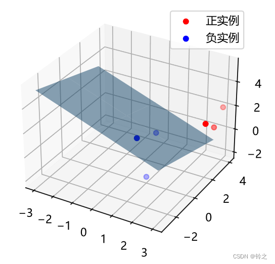
    def draw(self, X, y):
        # 分离正负实例点
        y = y[0]
        X_po = X[np.where(y == 1)]
        X_ne = X[np.where(y == 0)]
        # 绘制数据集散点图
        ax = plt.axes(projection='3d')
        x_1 = X_po[0, :]
        y_1 = X_po[1, :]
        z_1 = X_po[2, :]
        x_2 = X_ne[0, :]
        y_2 = X_ne[1, :]
        z_2 = X_ne[2, :]
        ax.scatter(x_1, y_1, z_1, c="r", label="正实例")
        ax.scatter(x_2, y_2, z_2, c="b", label="负实例")
        ax.legend(loc='best')
        # 绘制p=0.5的区分平面
        x = np.linspace(-3, 3, 3)
        y = np.linspace(-3, 3, 3)
        x_3, y_3 = np.meshgrid(x, y)
        a, b, c, d = self.w[0]
        z_3 = -(a * x_3 + b * y_3 + d) / c
        ax.plot_surface(x_3, y_3, z_3, alpha=0.5)  # 调节透明度
        plt.show()

# 训练数据集
X_train = np.array([[3, 3, 3], [4, 3, 2], [2, 1, 2], [1, 1, 1], [-1, 0, 1],
                    [2, -2, 1]])
y_train = np.array([[1, 1, 1, 0, 0, 0]])
# 构建实例，进行训练
clf = LogisticRegression()
clf.fit(X_train, y_train)
clf.draw(X_train, y_train)

迭代次数：3232次
最终梯度：[ 0.00144779  0.00046133  0.00490279 -0.00999848]
最终权重：[  2.96908597   1.60115396   5.04477438 -13.43744079]

在这里插入图片描述

文章参考：
李航《机器学习方法》
《统计学习方法》第二版的代码实现

铃之

关注

5
点赞
踩
7

收藏

觉得还不错? 一键收藏
0
评论
逻辑斯谛回归与最大熵模型的原理实现

逻辑斯谛回归(LR)是经典的分类方法1．逻辑斯谛回归模型是由以下条件概率分布表示的分类模型。逻辑斯谛回归模型可以用于二类或多类分类。PYk∣x1∑k1K−1expwk⋅xexpwk⋅xk12⋯K−1PYK∣x1∑k1K−1expwk⋅x1这里，x为输入特征，w为特征的权值。逻辑斯谛回归模型源自逻辑斯谛分布，其分布函数Fx是S形函数。
复制链接

扫一扫