


import numpy as np
import statsmodels.api as sm
import statsmodels.formula.api as smf
import matplotlib.pyplot as plt
import pandas as pd
from patsy import dmatrices
import scipy
from statsmodels.stats.outliers_influence import variance_inflation_factor
from itertools import combinations
import matplotlib.pyplot as plt
from mpl_toolkits.mplot3d import Axes3D
from statsmodels.stats.api import anova_lm
from sklearn.datasets import make_regression
from sklearn.linear_model import Ridge
from sklearn.metrics import mean_squared_error
df = pd.read_csv("C:\\Users\\33035\\Desktop\\data7.6.csv",encoding='gbk')
print(df)
#相关性矩阵
cor_matrix = df.corr(method='pearson')
print(cor_matrix)
#假设其为线性相关,找出不合理的地方
result = smf.ols('y~x1+x2+x3+x4',data=df).fit()
print(result.summary())
#两个方面:1.系数正负 2.模型显著性(f) 3.参数显著性(t)
## 一些方法的导入:
#1.求所有可能的变量组合
def comb(a):#参数a为所有自变量的列表
all=[]
for i in range(len(a)+1):
num_choose=i #从列表a中选num_choose个变量
combins=[c for c in combinations(a,num_choose)]
for i in combins:
i=list(i)
all.append(i)
return all
#2.对列表variables中的变量进行组合并建立模型,参数df为读入的数据
def buildModel(variables,df):
combine=''
for variable in variables:
combine=combine+variable+'+'#对列表中的变量进行组合
combine=combine[:-1]
if len(combine)==0:
combine='1'
result = smf.ols('y~'+combine,data=df).fit()#得出回归结果
return result
#3.变量列表和对应的aic以dataframe的形式输出
def printDataFrame(model,aic): #model为所有备选变量组合的列表,aic为所有备选模型aic的列表
data = {'model':model,'aic':aic}#输出Dataframe形式
frame = pd.DataFrame(data)
print(frame)
#4.所有子集回归
def allSubset(a,df):#参数a为所有自变量的列表,参数df为读入的数据
all=[]
all=comb(a)#先获取所有变量组合组合
aic=[] #保存所有aic值
for i in all:#遍历所有组合
result=buildModel(i,df) #对每一种组合建立模型
aic.append(result.aic)#获取aic并加入aic列表
printDataFrame(all,aic)
print("最小AIC为:{}".format(min(aic)))
index=aic.index(min(aic))
print("里面包含的自变量为:{}".format(all[index]))
temp=all[index] #获取最终变量组合
result=buildModel(temp,df)#输出最终的回归结果
print("回归结果:")
print(result.summary())
#前进法
def forward(a,df):
all=[]
all=comb(a)#求所有组合
start=[]
for i in range(len(all)):#把所有长度为0和长度为1的变量组合放入start列表中
if len(all[i])==0 or len(all[i])==1:
start.append(all[i])
#start=all[:len(a)+1]
while(len(start)>1):
#variables=[]
aic=[]
for i in start:#遍历所有组合
result=buildModel(i,df) #对每一种组合建立模型
aic.append(result.aic)
printDataFrame(start,aic) #输出
print("最小AIC为:{}".format(min(aic)))
index=aic.index(min(aic))
print("里面包含的自变量为:{}".format(start[index]))
temp=start[index]
if(index==0):#若aic最小的模型为起始模型则结束循环
break
start=[]
start.append(temp) #下一次循环的起始模型为上一次模型aic最小的模型,起始模型始终是列表的第一个元素
for i in all: #遍历所有变量组合,选取比起始变量组合多一个变量且拥有起始变量组合所有元素的变量组合
if len(i)==len(temp)+1 and set(temp) < set(i):
start.append(i)
print("*"*50)
result=buildModel(temp,df)#输出最终的回归结果
print("回归结果:")
print(result.summary())
#后退法
def backward(a,df):
all=[]
all=comb(a)#求所有组合
start=[]
for i in range(len(all)-1,-1,-1):#把所有长度为len(a)和长度为len(a)-1的变量组合放入start列表中
if len(all[i])==len(a) or len(all[i])==len(a)-1:
start.append(all[i])
while(len(start)>0):
aic=[]
for i in start:#遍历所有组合
result=buildModel(i,df) #对每一种组合建立模型
aic.append(result.aic)
printDataFrame(start,aic) #输出
print("最小AIC为:{}".format(min(aic)))
index=aic.index(min(aic))
print("里面包含的自变量为:{}".format(start[index]))
temp=start[index]
if(index==0):#若aic最小的模型为起始模型则结束循环
break
t=set(start[0]).difference(set(temp))
print("删减变量:{}".format(t))
start=[]#下一次循环的起始模型为上一次模型aic最小的模型
start.append(temp)
for i in all:
if len(i)==len(temp)-1 and set(temp) > set(i): #遍历所有变量组合,选取比起始变量组合少一个变量且所有变量都在起始变量组合中的变量组合
start.append(i)
print("*"*50)
result=buildModel(temp,df)#输出最终的回归结果
print("回归结果:")
print(result.summary())
#逐步回归法
def stepWise(a,df):
all=[]
dele=[]#可删减的变量列表
add=[]#可添加的变量列表
addOrDele=[]
var=[]
all=comb(a)#求所有组合
start=[]
for i in range(len(all)-1,-1,-1):#把所有长度为len(a)和长度为len(a)-1的变量组合放入start列表中
if len(all[i])==len(a) or len(all[i])==len(a)-1:
start.append(all[i])
while(1):
aic=[]
for i in start:#遍历所有组合
result=buildModel(i,df) #对每一种组合建立模型
aic.append(result.aic)
printDataFrame(start,aic) #输出
print("最小AIC为:{}".format(min(aic)))
index=aic.index(min(aic))
print("里面包含的自变量为:{}".format(start[index]))
temp=start[index]
if(index==0):#若aic最小的模型为起始模型则结束循环
break
if len(temp)>len(start[0]):#如果最小aic模型的变量组合长度大于起始模型,说明添加了变量
t=set(temp).difference(set(start[0]))
print("增加变量:{}".format(t))
addOrDele.append("+")
var.append(t)
if len(temp)<len(start[0]):#如果最小aic模型的变量组合长度小于起始模型,说明删减了变量
t=set(start[0]).difference(set(temp))
print("删减变量:{}".format(t))
addOrDele.append("-")
var.append(t)
start=[]
start.append(temp)
dele=[]
add=[]
for i in a:
if i in start[0]:
dele.append(i)
else:
add.append(i)
print("可增加的变量为:{}".format(add))
print("可删减的变量为:{}".format(dele))
#删除的情况
for i in all:#选取比起始变量组合多一个变量且拥有起始变量组合所有元素的变量组合
if len(i)==len(temp)-1 and set(temp) > set(i):
start.append(i)
#增加的情况
for i in all:#选取比起始变量组合少一个变量且所有变量都在起始变量组合中的变量组合
if len(i)==len(temp)+1 and set(temp) < set(i):
start.append(i)
print("*"*50)
data = {'':addOrDele,'d':var}#输出删减增加变量的情况
frame = pd.DataFrame(data)
print(frame)
result=buildModel(temp,df)#输出最终的回归结果
print("回归结果:")
print(result.summary())
##判断多重共线性:
# 1.方差扩大因子法
VIFlist = []
for i in range(1, 5, 1):
vif = variance_inflation_factor(result.model.exog, i) # 参数为设计矩阵和变量数
VIFlist.append(vif)
print('扩大因子法结果:\n',pd.Series(VIFlist))
## 检查出存在共线性后采取一下方法解决:
#1.消除一些变量(消除方法):
#1.1后退法:
a=['x1','x2','x3','x4']
backward(a,df)
#1.2逐步回归法
stepWise(a, df)
## 看看用了方法1之后是否还存在多重共线性(老规矩看一下线性回归两方面是否合理)
result1 = smf.ols('y~x1+x2+x4',data=df).fit()
print(result1.summary())
##好了很多,但是问题还没有解决,所以采用方法2
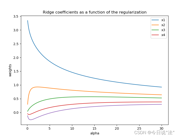
#方法2:岭回归(就是一个加了一个K值的有偏估计方法:原理还是最小二乘法,依然用OLS,目的是为了减少方差的不稳定性)
#步骤:
#0.构建未提出变量的岭回归模型
eps = list(np.random.randn(25)) # 误差项
y = -1.1584 + 0.0547 * df['x1'] + 0.1341 * df['x2'] -0.0548 * df['x3']-0.0320* df['x4'] + eps
df['y'] = y
print(df)
result = smf.ols('y~x1+x2+x3+x4', data=df).fit()
print(result.summary())
#1.获取数据k和peta
dfnorm = (df-df.mean())/df.std()
Xnorm = dfnorm.iloc[:, 1:]
ynorm = df.iloc[:, 0]
clf = Ridge()
coefs = []
errors = []
alphas = np.linspace(0.1, 30, 2000)
for a in alphas:
clf.set_params(alpha=a)
clf.fit(dfnorm, ynorm)
coefs.append(clf.coef_)
#查看数据:
plt.figure(figsize=(8, 6))
print(Xnorm.keys())
#2.画岭迹图
plt.subplot(111)
ax = plt.gca()
ax.plot(alphas, coefs, label=list(Xnorm.keys()))
ax.legend(list(Xnorm.keys()), loc='best')
plt.xlabel('alpha')
plt.ylabel('weights')
plt.title('Ridge coefficients as a function of the regularization')
plt.axis('tight')
plt.show()
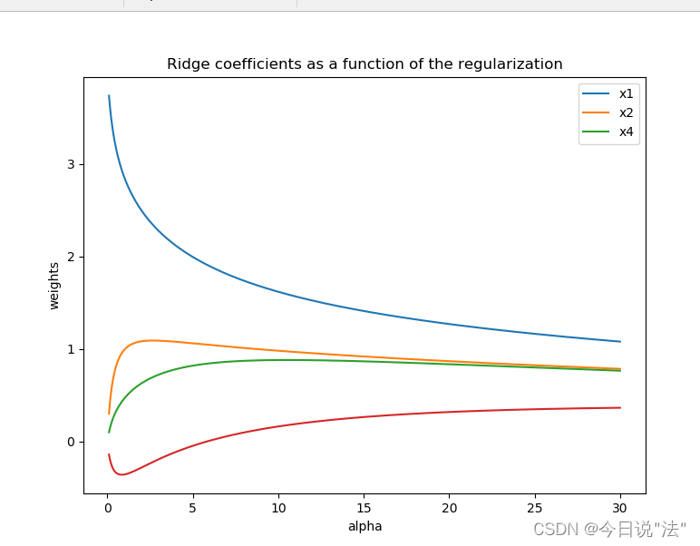
#构建剔除变量x3后的岭回归模型
result2 = smf.ols('y~x1+x2+x4', data=df).fit()
print(result.summary())
eps = list(np.random.randn(25)) # 误差项
y = -1.6214 + 0.0502 * df['x1'] + 0.1703 * df['x2']-0.0231 * df['x4'] + eps
# print(y)
df['y'] = y
print(df)
result = smf.ols('y~x1+x2+x4', data=df).fit()
print(result.summary())
dfnorm = (df - df.mean()) / df.std()
dfnorm = dfnorm.drop(['x3'],axis=1)
# 切片将x和y分开
Xnorm = dfnorm.iloc[:, 1:]
ynorm = df.iloc[:, 0]
clf = Ridge()
coefs = []
errors = []
alphas = np.linspace(0.1, 30, 2000)
for a in alphas:
clf.set_params(alpha=a)
clf.fit(dfnorm, ynorm)
#print(clf.coef_)
coefs.append(clf.coef_)
# 查看数据
plt.figure(figsize=(8, 6))
print(Xnorm.keys())
#画图
plt.subplot(111)
ax = plt.gca()
ax.plot(alphas, coefs, label=list(Xnorm.keys()))
# ax.set_xscale('log')
ax.legend(list(Xnorm.keys()), loc='best')
plt.xlabel('alpha')
plt.ylabel('weights')
plt.title('Ridge coefficients as a function of the regularization')
plt.axis('tight')
plt.show()y x1 x2 x3 x4
0 0.9 67.3 6.8 5 51.9
1 1.1 111.3 19.8 16 90.9
2 4.8 173.0 7.7 17 73.7
3 3.2 80.8 7.2 10 14.5
4 7.8 199.7 16.5 19 120.0
5 2.7 16.2 2.2 1 2.2
6 1.6 107.4 10.7 17 20.2
7 12.5 185.4 27.1 18 43.8
8 1.0 96.1 1.7 10 55.9
9 2.6 72.8 9.1 14 64.3
10 0.3 64.2 2.1 11 42.7
11 4.0 132.2 11.2 23 76.7
12 0.8 58.6 6.0 14 22.8
13 3.5 174.6 12.7 26 117.1
14 10.2 263.5 15.6 34 146.7
15 3.0 79.3 8.9 15 29.9
16 0.2 14.8 0.6 2 42.1
17 0.4 73.5 5.9 11 25.3
18 1.0 24.7 5.0 4 13.4
19 6.8 139.4 7.2 28 64.3
20 11.6 368.2 16.8 32 250.0
21 1.6 95.7 3.8 10 44.5
22 1.2 109.6 10.3 14 67.9
23 7.2 196.2 15.8 16 120.0
24 3.2 102.2 12.0 10 97.1
y x1 x2 x3 x4
y 1.000000 0.843571 0.731505 0.700281 0.642962
x1 0.843571 1.000000 0.678772 0.848416 0.891474
x2 0.731505 0.678772 1.000000 0.585831 0.535135
x3 0.700281 0.848416 0.585831 1.000000 0.717096
x4 0.642962 0.891474 0.535135 0.717096 1.000000
OLS Regression Results
==============================================================================
Dep. Variable: y R-squared: 0.803
Model: OLS Adj. R-squared: 0.764
Method: Least Squares F-statistic: 20.37
Date: Wed, 30 Nov 2022 Prob (F-statistic): 7.98e-07
Time: 20:43:24 Log-Likelihood: -46.749
No. Observations: 25 AIC: 103.5
Df Residuals: 20 BIC: 109.6
Df Model: 4
Covariance Type: nonrobust
==============================================================================
coef std err t P>|t| [0.025 0.975]
------------------------------------------------------------------------------
Intercept -1.1584 0.764 -1.517 0.145 -2.751 0.435
x1 0.0547 0.015 3.770 0.001 0.024 0.085
x2 0.1341 0.079 1.702 0.104 -0.030 0.298
x3 -0.0548 0.080 -0.684 0.502 -0.222 0.112
x4 -0.0320 0.015 -2.096 0.049 -0.064 -0.000
==============================================================================
Omnibus: 0.250 Durbin-Watson: 2.401
Prob(Omnibus): 0.882 Jarque-Bera (JB): 0.442
Skew: 0.045 Prob(JB): 0.802
Kurtosis: 2.355 Cond. No. 365.
==============================================================================Warnings:
[1] Standard Errors assume that the covariance matrix of the errors is correctly specified.
扩大因子法结果:
0 10.601022
1 1.940338
2 3.667517
3 5.234205
dtype: float64
model aic
0 [x1, x2, x3, x4] 103.498600
1 [x2, x3, x4] 114.919757
2 [x1, x3, x4] 104.879727
3 [x1, x2, x4] 102.076815
4 [x1, x2, x3] 106.461332
最小AIC为:102.07681497550593
里面包含的自变量为:['x1', 'x2', 'x4']
删减变量:{'x3'}
**************************************************
model aic
0 [x1, x2, x4] 102.076815
1 [x1, x2] 104.586108
2 [x1, x4] 103.408600
3 [x2, x4] 115.665323
最小AIC为:102.07681497550593
里面包含的自变量为:['x1', 'x2', 'x4']
回归结果:
OLS Regression Results
==============================================================================
Dep. Variable: y R-squared: 0.798
Model: OLS Adj. R-squared: 0.769
Method: Least Squares F-statistic: 27.71
Date: Wed, 30 Nov 2022 Prob (F-statistic): 1.71e-07
Time: 20:43:24 Log-Likelihood: -47.038
No. Observations: 25 AIC: 102.1
Df Residuals: 21 BIC: 107.0
Df Model: 3
Covariance Type: nonrobust
==============================================================================
coef std err t P>|t| [0.025 0.975]
------------------------------------------------------------------------------
Intercept -1.3841 0.680 -2.036 0.055 -2.798 0.030
x1 0.0487 0.011 4.263 0.000 0.025 0.073
x2 0.1346 0.078 1.730 0.098 -0.027 0.296
x4 -0.0303 0.015 -2.037 0.054 -0.061 0.001
==============================================================================
Omnibus: 0.159 Durbin-Watson: 2.470
Prob(Omnibus): 0.924 Jarque-Bera (JB): 0.374
Skew: -0.042 Prob(JB): 0.829
Kurtosis: 2.407 Cond. No. 327.
==============================================================================Warnings:
[1] Standard Errors assume that the covariance matrix of the errors is correctly specified.
model aic
0 [x1, x2, x3, x4] 103.498600
1 [x2, x3, x4] 114.919757
2 [x1, x3, x4] 104.879727
3 [x1, x2, x4] 102.076815
4 [x1, x2, x3] 106.461332
最小AIC为:102.07681497550593
里面包含的自变量为:['x1', 'x2', 'x4']
删减变量:{'x3'}
可增加的变量为:['x3']
可删减的变量为:['x1', 'x2', 'x4']
**************************************************
model aic
0 [x1, x2, x4] 102.076815
1 [x1, x2] 104.586108
2 [x1, x4] 103.408600
3 [x2, x4] 115.665323
4 [x1, x2, x3, x4] 103.498600
最小AIC为:102.07681497550593
里面包含的自变量为:['x1', 'x2', 'x4']
d
0 - {x3}
回归结果:
OLS Regression Results
==============================================================================
Dep. Variable: y R-squared: 0.798
Model: OLS Adj. R-squared: 0.769
Method: Least Squares F-statistic: 27.71
Date: Wed, 30 Nov 2022 Prob (F-statistic): 1.71e-07
Time: 20:43:24 Log-Likelihood: -47.038
No. Observations: 25 AIC: 102.1
Df Residuals: 21 BIC: 107.0
Df Model: 3
Covariance Type: nonrobust
==============================================================================
coef std err t P>|t| [0.025 0.975]
------------------------------------------------------------------------------
Intercept -1.3841 0.680 -2.036 0.055 -2.798 0.030
x1 0.0487 0.011 4.263 0.000 0.025 0.073
x2 0.1346 0.078 1.730 0.098 -0.027 0.296
x4 -0.0303 0.015 -2.037 0.054 -0.061 0.001
==============================================================================
Omnibus: 0.159 Durbin-Watson: 2.470
Prob(Omnibus): 0.924 Jarque-Bera (JB): 0.374
Skew: -0.042 Prob(JB): 0.829
Kurtosis: 2.407 Cond. No. 327.
==============================================================================Warnings:
[1] Standard Errors assume that the covariance matrix of the errors is correctly specified.
y x1 x2 x3 x4
0 1.926535 67.3 6.8 5 51.9
1 2.514286 111.3 19.8 16 90.9
2 5.343612 173.0 7.7 17 73.7
3 4.846388 80.8 7.2 10 14.5
4 7.202511 199.7 16.5 19 120.0
5 -0.287470 16.2 2.2 1 2.2
6 5.628303 107.4 10.7 17 20.2
7 10.463421 185.4 27.1 18 43.8
8 3.204158 96.1 1.7 10 55.9
9 1.391396 72.8 9.1 14 64.3
10 -1.160265 64.2 2.1 11 42.7
11 5.387054 132.2 11.2 23 76.7
12 0.773665 58.6 6.0 14 22.8
13 4.247559 174.6 12.7 26 117.1
14 9.467889 263.5 15.6 34 146.7
15 2.065919 79.3 8.9 15 29.9
16 -2.159934 14.8 0.6 2 42.1
17 2.649833 73.5 5.9 11 25.3
18 1.262153 24.7 5.0 4 13.4
19 3.788389 139.4 7.2 28 64.3
20 12.619581 368.2 16.8 32 250.0
21 2.848867 95.7 3.8 10 44.5
22 2.237317 109.6 10.3 14 67.9
23 7.741277 196.2 15.8 16 120.0
24 3.173480 102.2 12.0 10 97.1
OLS Regression Results
==============================================================================
Dep. Variable: y R-squared: 0.944
Model: OLS Adj. R-squared: 0.933
Method: Least Squares F-statistic: 84.08
Date: Wed, 30 Nov 2022 Prob (F-statistic): 3.24e-12
Time: 20:43:24 Log-Likelihood: -30.642
No. Observations: 25 AIC: 71.28
Df Residuals: 20 BIC: 77.38
Df Model: 4
Covariance Type: nonrobust
==============================================================================
coef std err t P>|t| [0.025 0.975]
------------------------------------------------------------------------------
Intercept -1.0699 0.401 -2.668 0.015 -1.906 -0.234
x1 0.0665 0.008 8.720 0.000 0.051 0.082
x2 0.1100 0.041 2.660 0.015 0.024 0.196
x3 -0.0940 0.042 -2.233 0.037 -0.182 -0.006
x4 -0.0396 0.008 -4.941 0.000 -0.056 -0.023
==============================================================================
Omnibus: 0.192 Durbin-Watson: 2.644
Prob(Omnibus): 0.908 Jarque-Bera (JB): 0.216
Skew: -0.172 Prob(JB): 0.898
Kurtosis: 2.702 Cond. No. 365.
==============================================================================Warnings:
[1] Standard Errors assume that the covariance matrix of the errors is correctly specified.
Index(['x1', 'x2', 'x3', 'x4'], dtype='object')


 6595
6595


 被折叠的 条评论
为什么被折叠?
被折叠的 条评论
为什么被折叠?
 到【灌水乐园】发言


