数学建模学习

ソ尛晴天づ_

已于 2022-07-18 10:27:41 修改

阅读量352

点赞数

分类专栏：学习笔记文章标签：学习 python

于 2022-07-18 10:16:10 首次发布

本文链接：https://blog.csdn.net/m0_56923407/article/details/125842292

版权

学习笔记专栏收录该内容

2 篇文章 0 订阅

订阅专栏

线性规划

线性规划标准型

在这里插入图片描述

求解函数

def linprog(c, A_ub=None, b_ub=None, A_eq=None, b_eq=None,
bounds=None, method=‘interior-point’, callback=None,
options=None, x0=None):

“”"
c:为目标函数
A_ub（可选参数）:不等式矩阵
b_ub（可选参数）:不等式常量向量
A_eq（可选参数）:等式矩阵
b_eq（可选参数）:等式常量向量
boundes（可选参数）：决策变量的范围默认为(0,None),格式为[(min,max),(min,max),…]，None表示无穷大
method（可选参数）:选择使用的算法，highs-ds、highs-ipm、highs、interior-point(默认)、revised simplex、simplex
x0（可选参数）：猜测决策变量的值
options（可选参数）：求解器选项字典
“”"

求解线性规划问题

求解：

max z=2x1+3x2-5x3

s.t. x1+x2+x3=7

2x1-x5+x3>=10

x1+3x2+x3<=12

x1,x2,x3>=0

import numpy as np
from scipy import optimize
import math
import sys

c=np.array([2,3,-5])
A=np.array([[-2,5,-1],[1,3,1]])
b=np.array([[-10,12]])
Aeq=np.array([[1,1,1]])
beq=np.array([[7]])
bounds=np.array([(0,None),(0,None),(0,None)])
res=optimize.linprog(c=-c,A_ub=A,b_ub=b,A_eq=Aeq,b_eq=beq)
print(res)
print("*********"*4)
print("最大值：",-res.fun)
print("x的值：",res.x)

     con: array([1.80714466e-09])
     fun: -14.571428565645034
 message: 'Optimization terminated successfully.'
     nit: 5
   slack: array([-2.24611441e-10,  3.85714286e+00])
  status: 0
 success: True
       x: array([6.42857143e+00, 5.71428571e-01, 2.35900788e-10])
************************************
最大值： 14.571428565645034
x的值： [6.42857143e+00 5.71428571e-01 2.35900788e-10]

可转成线性规划问题的问题

在这里插入图片描述

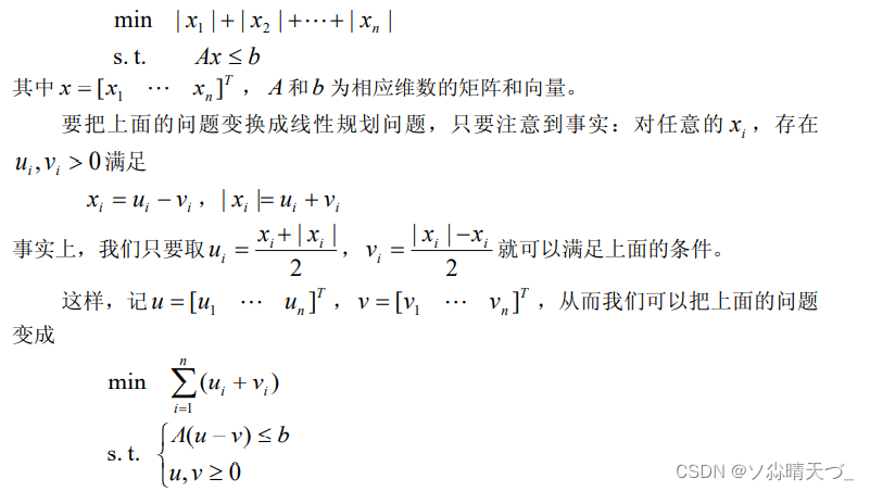
整数规划

分支定界算法

def integerPro(c, A=None, b=None, Aeq=None, beq=None,bounds=None, t=1.0E-8):
    res = optimize.linprog(c, A_ub=A, b_ub=b, A_eq=Aeq, b_eq=beq,bounds=bounds)
    bestVal = sys.maxsize
    bestX = res.x
    if not (type(res.x) is float or res.status != 0):
        bestVal = sum([x * y for x, y in zip(c, bestX)])
    if all(((x - math.floor(x)) <= t or (math.ceil(x) - x) <= t) for x in bestX):
        return (bestVal, bestX)
    else:
        ind = [i for i, x in enumerate(bestX) if (x - math.floor(x)) > t and (math.ceil(x) - x) > t][0]
        newCon1 = [0] * len(A[0])
        newCon2 = [0] * len(A[0])
        newCon1[ind] = -1
        newCon2[ind] = 1
        newA1 = A.copy()
        newA2 = A.copy()
        newA1.append(newCon1)
        newA2.append(newCon2)
        newB1 = b.copy()
        newB2 = b.copy()
        newB1.append(-math.ceil(bestX[ind]))
        newB2.append(math.floor(bestX[ind]))
        r1 = integerPro(c, newA1, newB1, Aeq, beq,bounds)
        r2 = integerPro(c, newA2, newB2, Aeq, beq,bounds)
        if r1[0] < r2[0]:
            return r1
        else:
            return r2

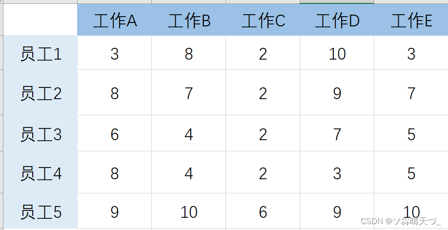
指派问题

在这里插入图片描述

import numpy as np
from scipy import optimize
import math
import sys

cost_matrix = np.array([[3, 8, 2, 10, 3],
                        [8, 7, 2, 9, 7],
                        [6, 4, 2, 7, 5],
                        [8, 4, 2, 3, 5],
                        [9, 10, 6, 9, 10]])

row_ind,col_ind = optimize.linear_sum_assignment(cost_matrix, False)
print(row_ind)#行
print(col_ind)#列
print(cost_matrix[[row_ind],[col_ind]].sum())

[0 1 2 3 4]
[4 2 1 3 0]
21

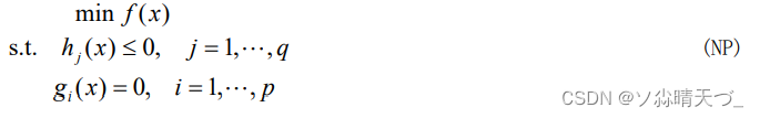
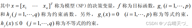
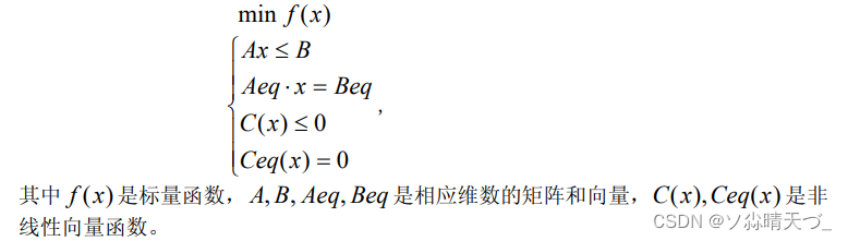
非线性规划

非线性规划一般形式

非线性规划标准型

求解函数

def minimize(fun, x0, args=(), method=None, jac=None, hess=None,
hessp=None, bounds=None, constraints=(), tol=None,
callback=None, options=None)

fun:目标函
x0:初始猜测值
args（可选择参数）:常量
bounds（可选择参数）:范围[(min,max),…]
method（可选择参数）:选择求解方法
constraints（可选择参数）：约束条件，eq表示函数结果等于0 ； ineq 表示表达式大于等于0

在这里插入图片描述


import numpy as np
from scipy import optimize
import math
import sys

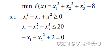
#目标函数
def fun(x):
    return x[0] ** 2 + x[1] ** 2 + x[2] ** 2 + 8

 #约束
constraints = [
    {"type": "ineq", "fun": lambda x: x[0] ** 2 - x[1] + x[2] ** 2},
    {"type": "ineq", "fun": lambda x: -(x[0] + x[1] ** 2 + x[2] ** 2 - 20)},
    {"type": "eq", "fun": lambda x: -x[0] - x[1] ** 2 + 2},
    {"type": "eq", "fun": lambda x: x[1] + 2 * x[2] ** 2 - 3}
]
x0 = (0, 0, 0) #猜测值
bounds = ((0, None) for i in range(3)) #范围

res = optimize.minimize(fun, x0, bounds=bounds, constraints=constraints)

print(res)

     fun: 10.651091840572583
     jac: array([1.10433471, 2.40651834, 1.89564812])
 message: 'Optimization terminated successfully'
    nfev: 71
     nit: 15
    njev: 15
  status: 0
 success: True
       x: array([0.55216734, 1.20325918, 0.94782404])

或者加上args参数，将常数写args里面

args=[8]
#目标函数
def fun(x,args):
    return x[0] ** 2 + x[1] ** 2 + x[2] ** 2 + args[0]

 #约束
constraints = [
    {"type": "ineq", "fun": lambda x: x[0] ** 2 - x[1] + x[2] ** 2},
    {"type": "ineq", "fun": lambda x: -(x[0] + x[1] ** 2 + x[2] ** 2 - 20)},
    {"type": "eq", "fun": lambda x: -x[0] - x[1] ** 2 + 2},
    {"type": "eq", "fun": lambda x: x[1] + 2 * x[2] ** 2 - 3}
]
x0 = (0, 0, 0) #猜测值
bounds = ((0, None) for i in range(3)) #范围

res = optimize.minimize(fun, x0,args=args, bounds=bounds, constraints=constraints)

print(res)

     fun: 10.651091840572583
     jac: array([1.10433471, 2.40651834, 1.89564812])
 message: 'Optimization terminated successfully'
    nfev: 71
     nit: 15
    njev: 15
  status: 0
 success: True
       x: array([0.55216734, 1.20325918, 0.94782404])

动态规划

以后补充

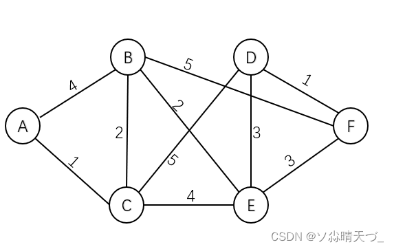
图与网络

最短路径

dijkstra算法

from math import inf

node_name = ['A', 'B', 'C', 'D', 'E', 'F']
# 邻接矩阵
map = [[0, 4, 1, inf, inf, inf],
       [4, 0, 2, inf, 2, 5],
       [1, 2, 0, 5, 4, inf],
       [inf, inf, 5, 0, 3, 1],
       [inf, 2, 4, 3, 0, 3],
       [inf, 5, inf, 1, 3, 0]]

dist = [inf for i in range(len(map))]
path = [-1 for i in range(len(map))]
S = [0 for i in range(len(map))]

#起始点u
def dijkstra(u):
    for i in range(len(map)):
        dist[i] = map[u][i]
        if dist[i] != inf:
            path[i] = u

    S[u] = 1

    for i in range(len(map) - 1):
        temp = inf
        t = u
        for j in range(len(map)):
            if S[j] != 1 and dist[j] < temp:
                t = j
                temp = dist[j]

        if t == u:
            return
        S[t] = 1

        for j in range(len(map)):
            if S[j] != 1 and dist[j] > dist[t] + map[t][j]:
                dist[j] = dist[t] + map[t][j]
                path[j] = t


def printPath():
    for i in range(len(map)):
        num = path[i]
        p = node_name[i] + '->'
        if num != -1:
            while num != 0:
                p += node_name[num] + '->'
                num = path[num]
        p += 'A'
        print("路径：",p,"长度：",dist[i])


dijkstra(0)
printPath()

路径： A->A 长度： 0
路径： B->C->A 长度： 3
路径： C->A 长度： 1
路径： D->C->A 长度： 6
路径： E->C->A 长度： 5
路径： F->D->C->A 长度： 7

floyd算法

from math import inf

node_name = ['A', 'B', 'C', 'D', 'E', 'F']

# 邻接矩阵
map = [[0, 4, 1, inf, inf, inf],
       [4, 0, 2, inf, 2, 5],
       [1, 2, 0, 5, 4, inf],
       [inf, inf, 5, 0, 3, 1],
       [inf, 2, 4, 3, 0, 3],
       [inf, 5, inf, 1, 3, 0]]

dist = map.copy()
path = [[-1 for i in range(len(map))] for j in range(len(map))]


def floyd():
    for k in range(len(map)):
        for i in range(len(map)):
            for j in range(len(map)):
                if dist[i][j] > dist[i][k] + dist[k][j]:
                    dist[i][j] = dist[i][k] + dist[k][j]
                    path[i][j] = k


def findPath(start, end):
    if dist[start][end] < inf and path[start][end] == -1:
        print('->{}'.format(node_name[end]),end='')
    else:
        mid = path[start][end]
        findPath(start, mid)
        findPath(mid, end)


def printPath(start,end):
    print(node_name[start],end='')
    findPath(start,end)
    print(' 最短路径长度为：',dist[start][end])

floyd()
#A到F的路径
printPath(0,5)

A->C->D->F 最短路径长度为： 7

最小生成树

prim

from math import inf

node_name = ['A', 'B', 'C', 'D', 'E', 'F']

# 邻接矩阵
map = [[0, 4, 1, inf, inf, inf],
       [4, 0, 2, inf, 2, 5],
       [1, 2, 0, 5, 4, inf],
       [inf, inf, 5, 0, 3, 1],
       [inf, 2, 4, 3, 0, 3],
       [inf, 5, inf, 1, 3, 0]]
# 节点个数
n = len(map)
dist = [inf for i in range(n)]
S = [0 for i in range(n)]
path = [-1 for i in range(n)]


# v是开始结点
def prim(v):
    for i in range(n):
        dist[i] = map[v][i]
        if map[v][i] != inf:
            path[i] = v
    S[v] = 1

    for i in range(n - 1):
        min = inf
        t = v
        for j in range(n):
            if S[j] != 1 and min > dist[j]:
                min = dist[j]
                t = j

        S[t] = 1
        print(node_name[path[t]], '->', node_name[t])

        for j in range(n):
            if S[j] != 1 and dist[j] > map[t][j]:
                dist[j] = map[t][j]
                path[j] = t


prim(0)
if sum(dist) == inf:
    print("无法生成最小生成树")
else:
    print("最小权值:", sum(dist))

A -> C
C -> B
B -> E
E -> D
D -> F
最小权值: 9

kruskal

以后补充

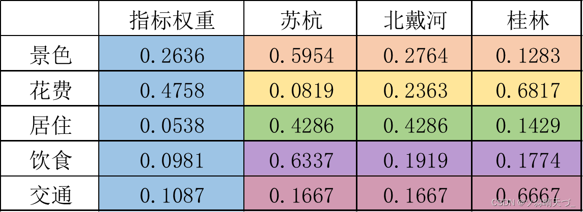
层次分析

参考：https://blog.csdn.net/weixin_43819566/article/details/112251317

import numpy as np

n = 5
RI = [0, 0, 0.52, 0.89, 1.12, 1.26, 1.36, 1.41, 1.46, 1.49, 1.52, 1.54, 1.56, 1.58, 1.59]
# 选择旅游地
A = np.array([[1, 1 / 2, 4, 3, 3],
              [2, 1, 7, 5, 5],
              [1 / 4, 1 / 7, 1, 1 / 2, 1 / 3],
              [1 / 3, 1 / 5, 2, 1, 1],
              [1 / 3, 1 / 5, 3, 1, 1]])
# 景色
B1 = np.array([[1, 2, 5],
               [1 / 2, 1, 2],
               [1 / 5, 1 / 2, 1]])
# 花费
B2 = np.array([[1, 1 / 3, 1 / 8],
               [3, 1, 1 / 3],
               [8, 3, 1]])
# 居住
B3 = np.array([[1, 1, 3],
               [1, 1, 3],
               [1 / 3, 1 / 3, 1]])
# 饮食
B4 = np.array([[1, 3, 4],
               [1 / 3, 1, 1],
               [1 / 4, 1, 1]])
# 交通
B5 = np.array([[1, 1, 1 / 4],
               [1, 1, 1 / 4],
               [4, 4, 1]])

matrixs = [A, B1, B2, B3, B4, B5]

res = np.zeros((5, 4))

for i in range(len(matrixs)):
    # 求解特征值和特征向量
    res1 = np.linalg.eig(matrixs[i])
    # 特征值
    v = res1[0][0]
    # 权重向量
    w = res1[1][:, 0]
    # 权重向量归一化
    w = w / sum(w)

    CI = (v - n) / (n - 1)

    CR = CI / RI[n - 1]
    # print(v)
    # print(w)

    if i == 0:
        res[:, 0] = w
    else:
        res[i - 1, 1:] = w

#权重矩阵
print(res)

score = []

for i in range(res.shape[1] - 1):
    score.append(np.sum(res[:, 0] * res[:, i + 1]))
print("苏杭得分：",score[0])
print("北戴河得分：",score[1])
print("桂林得分：",score[2])

[[0.26360349 0.59537902 0.27635046 0.12827052]
 [0.47583538 0.08193475 0.2363407  0.68172455]
 [0.0538146  0.42857143 0.42857143 0.14285714]
 [0.09806829 0.63370792 0.19192062 0.17437146]
 [0.10867824 0.16666667 0.16666667 0.66666667]]
苏杭得分： 0.2992545297453049
北戴河得分： 0.24530398001537013
桂林得分： 0.4554414902393249

灰色关联度分析

系统分析

参考：https://blog.csdn.net/weixin_43819566/article/details/112914383

下表为某地区国内生产总值的统计数据（以百万元计），问该地区从 2000 年到 2005 年之间，哪一种产业对 GDP 总量影响最大。
在这里插入图片描述

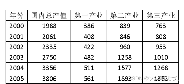
import numpy as np

x = np.array([[1988, 386, 839, 763],
              [2061, 408, 846, 808],
              [2335, 422, 960, 953],
              [2750, 482, 1258, 1010],
              [3356, 511, 1577, 1268],
              [3806, 561, 1893, 1352]], dtype='float')

average = x.mean(axis=0)

# 分辨系数
p = 0.5

for i in range(x.shape[1]):
    x[:, i] = x[:, i] / average[i]

y = np.zeros((x.shape[0], x.shape[1] - 1))

# 得到差值矩阵
for i in range(x.shape[1] - 1):
    y[:, i] = np.abs(x[:, i + 1] - x[:, 0])

# 两级最小差
a = y.min()
# 两级最大差
b = y.max()

# 得到关联系数矩阵
y = (a + p * b) / (y + p * b)

r=y.mean(axis=0)

print("关联系数矩阵")
print(y)
print("关联度")
print(r)

关联系数矩阵
[[0.4751452  0.6586359  0.89222807]
 [0.42986317 0.57328932 0.76795519]
 [0.63557702 0.54618164 0.57663015]
 [0.75204756 0.89847974 0.7752663 ]
 [0.42237767 0.66568635 1.        ]
 [0.33558385 0.40350205 0.53171804]]
关联度
[0.50843241 0.62429583 0.75729962]

综合评价

1、对指标进行正向化

2、对正向化矩阵进行预处理

3、将预处理后的具有真每一行取出最大值构成母序列

4、计算各个指标与母序列的灰色关联度

5、计算各个指标的权重

6、计算每个评价对象的得分

灰色预测

参考：https://blog.csdn.net/weixin_43819566/article/details/113819188

预测计算

在这里插入图片描述

import numpy as np
from numpy.linalg import inv
from math import e

x0 = np.array([71.1, 72.4, 72.4, 72.1, 71.4, 72.0, 71.6])
print("参考数据：", x0)
n = x0.shape[0]
# 求级比
jibi = np.array([x0[i] / x0[i + 1] for i in range(n - 1)])
print("级比：", jibi)
# 可容覆盖区间
X = (pow(e, -2 / (n + 1)), pow(e, 2 / (n + 1)))

# 校验级比是否都在可容覆盖区间
if np.min(jibi) >= X[0] and np.max(jibi) <= X[1]:
    print("级比都落在可容覆盖区间,通过级比检验")
else:
    print("不满足条件")

# GM(1,1)建模
# 原始数据累加
x1 = np.array([np.sum(x0[:i + 1]) for i in range(n)])
print("累加生成数列", x1)
Z = np.array([0.5 * x1[i] + 0.5 * x1[i + 1] for i in range(n - 1)])
print(Z)

B = np.ones((n - 1, 2), dtype=float)
B[:, 0] = -Z

Y = x0[1:].reshape((n - 1, 1))
"""
u=(a,b)T=(BTB)-1BTY
"""
u = inv((B.T @ B)) @ B.T @ Y
a, b = u[0, 0], u[1, 0]
print("a=", a, "b=", b)

# 预测值
# 需要预测的数量
count = n
res = []
x2 = np.array([(x0[0] - b / a) * pow(e, -a * k) + b / a for k in range(count)])
res.append(x2[0])
for i in range(1, count):
    res.append(x2[i]-x2[i-1])
res=np.array(res)
print("预测值:", np.round(res,4))

# 检验
# 残差检验

cancha=[1-res[i]/x0[i] for i in range(n)]
print("残差：",cancha)
if max(cancha)<0.1:
    print("达到较高要求")
#

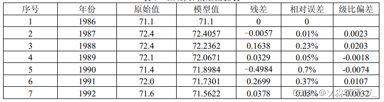
参考数据： [71.1 72.4 72.4 72.1 71.4 72.  71.6]
级比： [0.9820442  1.         1.00416089 1.00980392 0.99166667 1.00558659]
级比都落在可容覆盖区间,通过级比检验
累加生成数列 [ 71.1 143.5 215.9 288.  359.4 431.4 503. ]
[107.3  179.7  251.95 323.7  395.4  467.2 ]
a= 0.0023437864785236795 b= 72.65726960367881
预测值: [71.1    72.4057 72.2362 72.0671 71.8984 71.7301 71.5622]
残差： [2.042810365310288e-14, -7.930166340575084e-05, 0.002261925940694187, 0.0004559153760241852, -0.006980620867546694, 0.003748623322583966, 0.0005282688652282763]
达到较高要求

插值

拉格朗日多项式插值

避免Runge现象的常用方法是：将插值区间分成诺干小区间，在小区间内用低次（二次，三次）插值，既分段低次插值

给出结点x0=-1,x1=1,x2=2处的函数值为y0=2,y1=1,y2=3,要求计算出它的拉格朗日插值多项式，并计算f(0.5)的值

def lagrange(x0, y0, x):
    y = []
    for i in range(len(x)):
        s = 0
        for j in range(len(x0)):
            p = 1
            for k in range(len(x0)):
                if j != k:
                    p *= (x[i] - x0[k]) / (x0[j] - x0[k])
            s += p * y0[j]
        y.append(s)
    return y


x0 = [-1, 1, 2]
y0 = [2, 1, 3]
x = [0.5]
print(lagrange(x0, y0, x))

[0.625]

import numpy as np
from matplotlib import pyplot as plt

plt.rcParams['font.sans-serif'] = ['SimHei']  # 用来正常显示中文标签
plt.rcParams['axes.unicode_minus'] = False  # 用来正常显示负号

x0 = np.arange(-np.pi, np.pi, 1)  # 定义样本点X，从-pi到pi每次间隔1
y0 = np.sin(x0)  # 定义样本点Y，形成sin函数

x = np.arange(-np.pi, np.pi, 0.1)
y = np.array(lagrange(x0, y0, x))

plt.plot(x0, y0, 'o', label='样本点')
plt.plot(x, y, label="插值点")
plt.yticks(ticks=[-1.5+i*0.25 for i in range(13)])
plt.title('拉格朗日插值')
plt.legend()

plt.show()

在这里插入图片描述

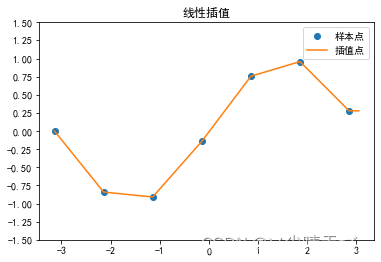
分段线性插值

import numpy as np
from matplotlib import pyplot as plt


x = range(0, 26, 2)
y = [12, 9, 9, 10, 18, 24, 28, 27, 25, 20, 18, 15, 13]
x1 = 13

y1 = np.interp(x1, x, y)
print((x1,y1))

(13, 27.5)

import numpy as np
from matplotlib import pyplot as plt

plt.rcParams['font.sans-serif'] = ['SimHei']  # 用来正常显示中文标签
plt.rcParams['axes.unicode_minus'] = False  # 用来正常显示负号

x = np.arange(-np.pi, np.pi, 1)  # 定义样本点X，从-pi到pi每次间隔1
y = np.sin(x)  # 定义样本点Y，形成sin函数

x1 = np.arange(-np.pi, np.pi, 0.1)
y1 = np.interp(x1, x, y)

plt.plot(x,y,'o',label='样本点')
plt.plot(x1,y1,label="插值点")
plt.yticks(ticks=[-1.5+i*0.25 for i in range(13)])
plt.title('线性插值')
plt.legend()

plt.show()

在这里插入图片描述

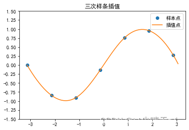
三次样条插值

三次样条插值更加的圆滑

import scipy.interpolate as spi
import numpy as np
from matplotlib import pyplot as plt

plt.rcParams['font.sans-serif'] = ['SimHei']  # 用来正常显示中文标签
plt.rcParams['axes.unicode_minus'] = False  # 用来正常显示负号

x = np.arange(-np.pi, np.pi, 1)  # 定义样本点X，从-pi到pi每次间隔1
y = np.sin(x)  # 定义样本点Y，形成sin函数

x1 = np.arange(-np.pi, np.pi, 0.1)

ipo = spi.splrep(x, y, k=3)  # 样本点导入，生成参数
y1 = spi.splev(x1, ipo)  # 根据观测点和样条参数，生成插值

plt.plot(x,y,'o',label='样本点')
plt.plot(x1,y1,label="插值点")
plt.yticks(ticks=[-1.5+i*0.25 for i in range(13)])
plt.title('三次样条插值')
plt.legend()

plt.show()