


文章目录
一、实现卷积-池化-激活

可视化卷积核和特征图
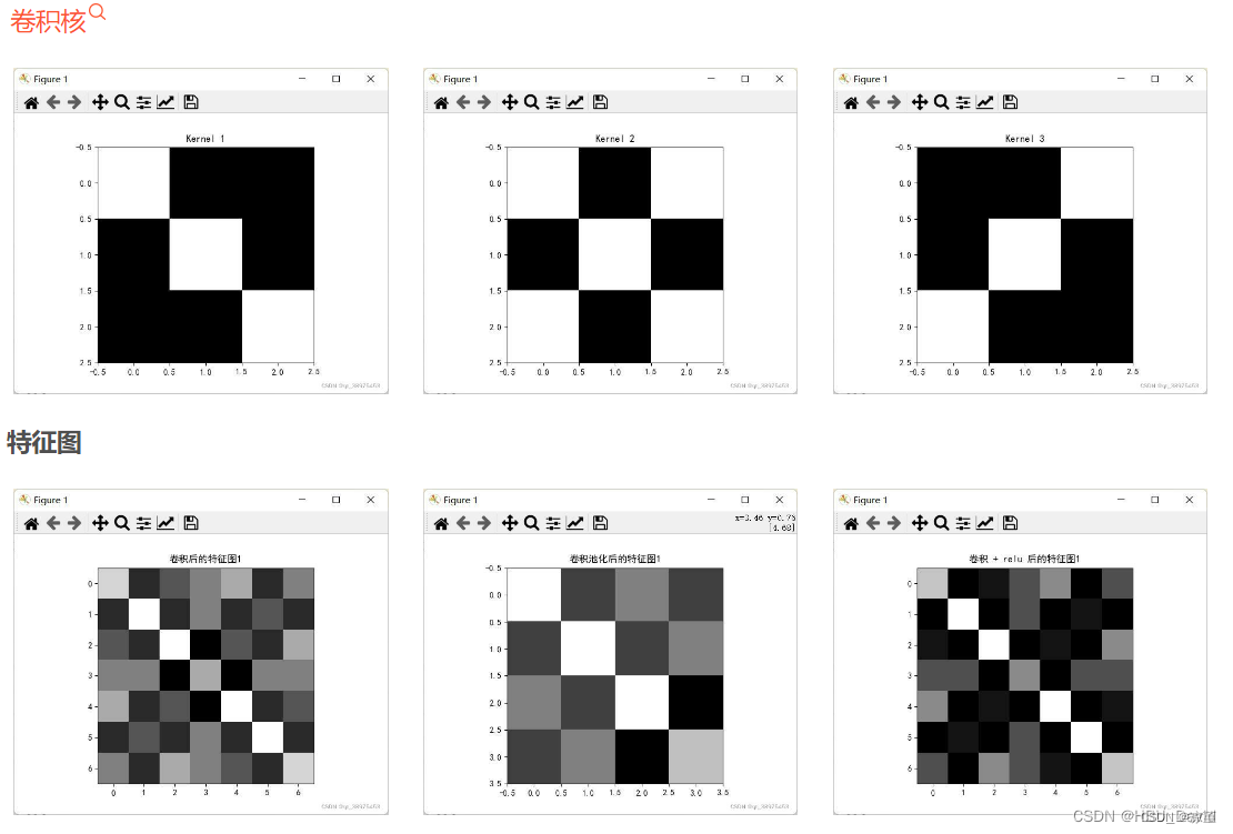
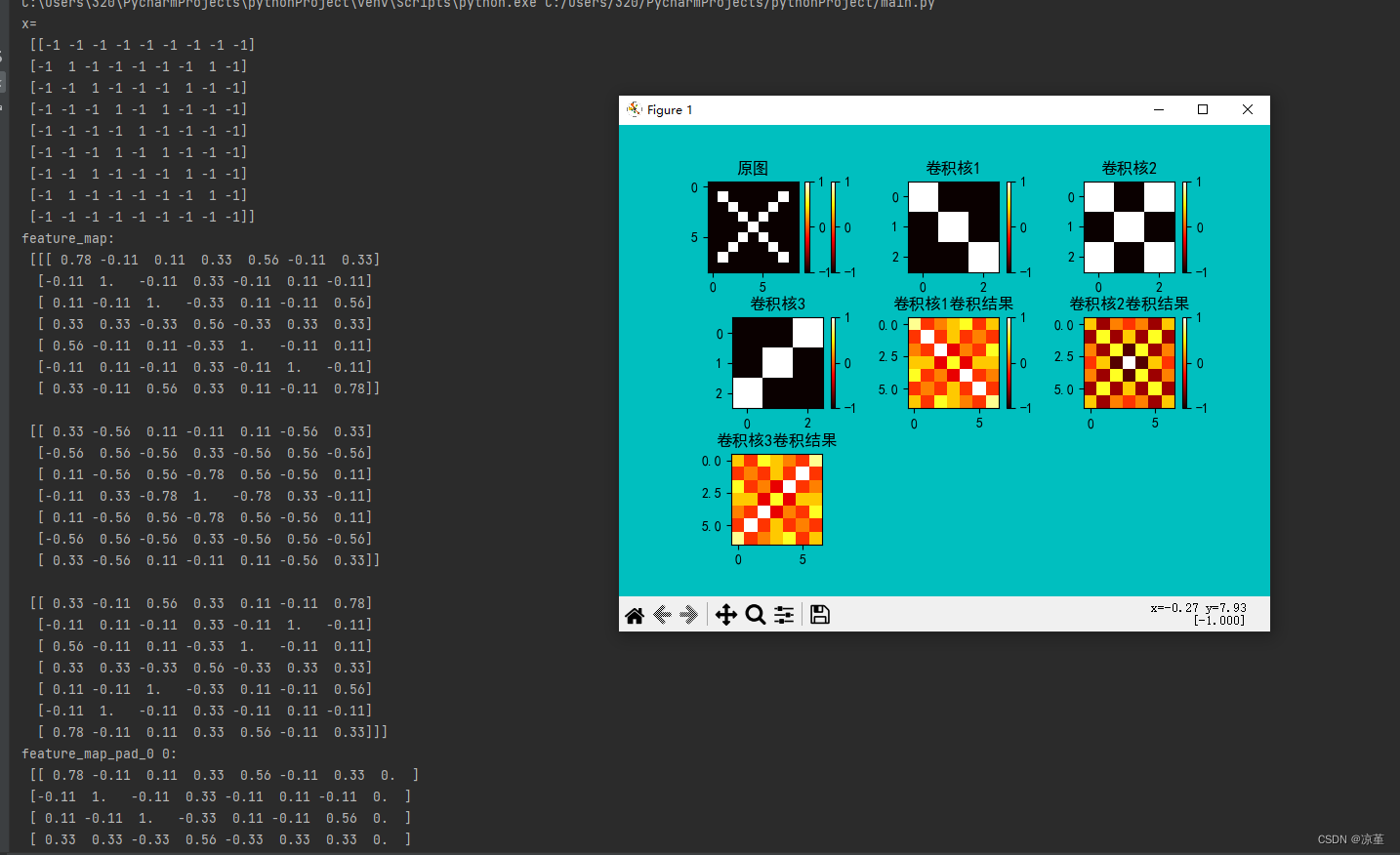
1. Numpy版本:手工实现 卷积-池化-激活
自定义卷积算子、池化算子实现
代码如下:
import numpy as np
import matplotlib.pyplot as plt
plt.rcParams['font.sans-serif'] = ['SimHei'] # 用来正常显示中文标签
plt.rcParams['axes.unicode_minus'] = False # 用来正常显示负号
x = np.array([[-1, -1, -1, -1, -1, -1, -1, -1, -1],
[-1, 1, -1, -1, -1, -1, -1, 1, -1],
[-1, -1, 1, -1, -1, -1, 1, -1, -1],
[-1, -1, -1, 1, -1, 1, -1, -1, -1],
[-1, -1, -1, -1, 1, -1, -1, -1, -1],
[-1, -1, -1, 1, -1, 1, -1, -1, -1],
[-1, -1, 1, -1, -1, -1, 1, -1, -1],
[-1, 1, -1, -1, -1, -1, -1, 1, -1],
[-1, -1, -1, -1, -1, -1, -1, -1, -1]])
print("x=\n", x)
# 初始化 三个 卷积核
Kernel = [[0 for i in range(0, 3)] for j in range(0, 3)]
Kernel[0] = np.array([[1, -1, -1],
[-1, 1, -1],
[-1, -1, 1]])
Kernel[1] = np.array([[1, -1, 1],
[-1, 1, -1],
[1, -1, 1]])
Kernel[2] = np.array([[-1, -1, 1],
[-1, 1, -1],
[1, -1, -1]])
plt.figure(1, figsize=[50, 50], edgecolor='c', facecolor='c')
plt.subplots_adjust(left=None, bottom=None, right=None, top=None, wspace=0.15, hspace=0.5)
plt.subplot(331).set_title('原图')
plt.imshow(x, cmap=plt.cm.hot, vmin=-1, vmax=1)
plt.colorbar()
plt.subplot(332).set_title('卷积核1')
plt.colorbar()
plt.imshow(Kernel[0], cmap=plt.cm.hot, vmin=-1, vmax=1)
plt.subplot(333).set_title('卷积核2')
plt.colorbar()
plt.imshow(Kernel[1], cmap=plt.cm.hot, vmin=-1, vmax=1)
plt.subplot(334).set_title('卷积核3')
plt.colorbar()
plt.imshow(Kernel[2], cmap=plt.cm.hot, vmin=-1, vmax=1)
# --------------- 卷积 ---------------
stride = 1 # 步长
feature_map_h = 7 # 特征图的高
feature_map_w = 7 # 特征图的宽
feature_map = [0 for i in range(0, 3)] # 初始化3个特征图
for i in range(0, 3):
feature_map[i] = np.zeros((feature_map_h, feature_map_w)) # 初始化特征图
for h in range(feature_map_h): # 向下滑动,得到卷积后的固定行
for w in range(feature_map_w): # 向右滑动,得到卷积后的固定行的列
v_start = h * stride # 滑动窗口的起始行(高)
v_end = v_start + 3 # 滑动窗口的结束行(高)
h_start = w * stride # 滑动窗口的起始列(宽)
h_end = h_start + 3 # 滑动窗口的结束列(宽)
window = x[v_start:v_end, h_start:h_end] # 从图切出一个滑动窗口
for i in range(0, 3):
feature_map[i][h, w] = np.divide(np.sum(np.multiply(window, Kernel[i][:, :])), 9)
print("feature_map:\n", np.around(feature_map, decimals=2))
plt.subplot(335).set_title('卷积核1卷积结果')
plt.colorbar()
plt.imshow(feature_map[0], cmap=plt.cm.hot, vmin=-1, vmax=1)
plt.subplot(336).set_title('卷积核2卷积结果')
plt.colorbar()
plt.imshow(feature_map[1], cmap=plt.cm.hot, vmin=-1, vmax=1)
plt.subplot(337).set_title('卷积核3卷积结果')
plt.colorbar()
plt.imshow(feature_map[2], cmap=plt.cm.hot, vmin=-1, vmax=1)
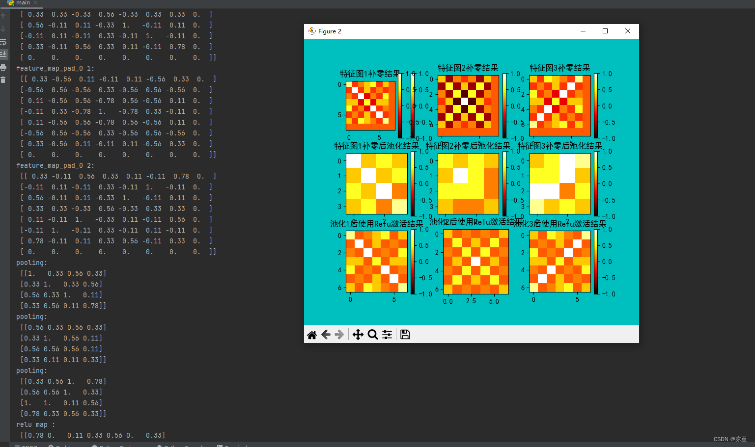
# --------------- 池化 ---------------
pooling_stride = 2 # 步长
pooling_h = 4 # 特征图的高
pooling_w = 4 # 特征图的宽
feature_map_pad_0 = [[0 for i in range(0, 8)] for j in range(0, 8)]
for i in range(0, 3): # 特征图 补 0 ,行 列 都要加 1 (因为上一层是奇数,池化窗口用的偶数)
feature_map_pad_0[i] = np.pad(feature_map[i], ((0, 1), (0, 1)), 'constant', constant_values=(0, 0))
print("feature_map_pad_0 0:\n", np.around(feature_map_pad_0[0], decimals=2))
print("feature_map_pad_0 1:\n", np.around(feature_map_pad_0[1], decimals=2))
print("feature_map_pad_0 2:\n", np.around(feature_map_pad_0[2], decimals=2))
plt.figure(2, figsize=[50, 50], edgecolor='c', facecolor='c')
plt.subplot(331).set_title('特征图1补零结果')
plt.imshow(feature_map_pad_0[0], cmap=plt.cm.hot, vmin=-1, vmax=1)
plt.colorbar()
plt.subplot(332).set_title('特征图2补零结果')
plt.colorbar()
plt.imshow(feature_map_pad_0[1], cmap=plt.cm.hot, vmin=-1, vmax=1)
plt.subplot(333).set_title('特征图3补零结果')
plt.colorbar()
plt.imshow(feature_map_pad_0[2], cmap=plt.cm.hot, vmin=-1, vmax=1)
pooling = [0 for i in range(0, 3)]
for i in range(0, 3):
pooling[i] = np.zeros((pooling_h, pooling_w)) # 初始化特征图
for h in range(pooling_h): # 向下滑动,得到卷积后的固定行
for w in range(pooling_w): # 向右滑动,得到卷积后的固定行的列
v_start = h * pooling_stride # 滑动窗口的起始行(高)
v_end = v_start + 2 # 滑动窗口的结束行(高)
h_start = w * pooling_stride # 滑动窗口的起始列(宽)
h_end = h_start + 2 # 滑动窗口的结束列(宽)
for i in range(0, 3):
pooling[i][h, w] = np.max(feature_map_pad_0[i][v_start:v_end, h_start:h_end])
print("pooling:\n", np.around(pooling[0], decimals=2))
print("pooling:\n", np.around(pooling[1], decimals=2))
print("pooling:\n", np.around(pooling[2], decimals=2))
plt.subplot(334).set_title('特征图1补零后池化结果')
plt.colorbar()
plt.imshow(pooling[0], cmap=plt.cm.hot, vmin=-1, vmax=1)
plt.subplot(335).set_title('特征图2补零后池化结果')
plt.colorbar()
plt.imshow(pooling[1], cmap=plt.cm.hot, vmin=-1, vmax=1)
plt.subplot(336).set_title('特征图3补零后池化结果')
plt.colorbar()
plt.imshow(pooling[2], cmap=plt.cm.hot, vmin=-1, vmax=1)
# --------------- 激活 ---------------
def relu(x):
return (abs(x) + x) / 2
relu_map_h = 7 # 特征图的高
relu_map_w = 7 # 特征图的宽
relu_map = [0 for i in range(0, 3)] # 初始化3个特征图
for i in range(0, 3):
relu_map[i] = np.zeros((relu_map_h, relu_map_w)) # 初始化特征图
for i in range(0, 3):
relu_map[i] = relu(feature_map[i])
print("relu map :\n", np.around(relu_map[0], decimals=2))
print("relu map :\n", np.around(relu_map[1], decimals=2))
print("relu map :\n", np.around(relu_map[2], decimals=2))
plt.subplot(337).set_title('池化1后使用Relu激活结果')
plt.colorbar()
plt.imshow(relu_map[0], cmap=plt.cm.hot, vmin=-1, vmax=1)
plt.subplot(338).set_title('池化2后使用Relu激活结果')
plt.colorbar()
plt.imshow(relu_map[1], cmap=plt.cm.hot, vmin=-1, vmax=1)
plt.subplot(339).set_title('池化3后使用Relu激活结果')
plt.imshow(relu_map[2], cmap=plt.cm.hot, vmin=-1, vmax=1)
plt.colorbar()
plt.show()
运行结果:

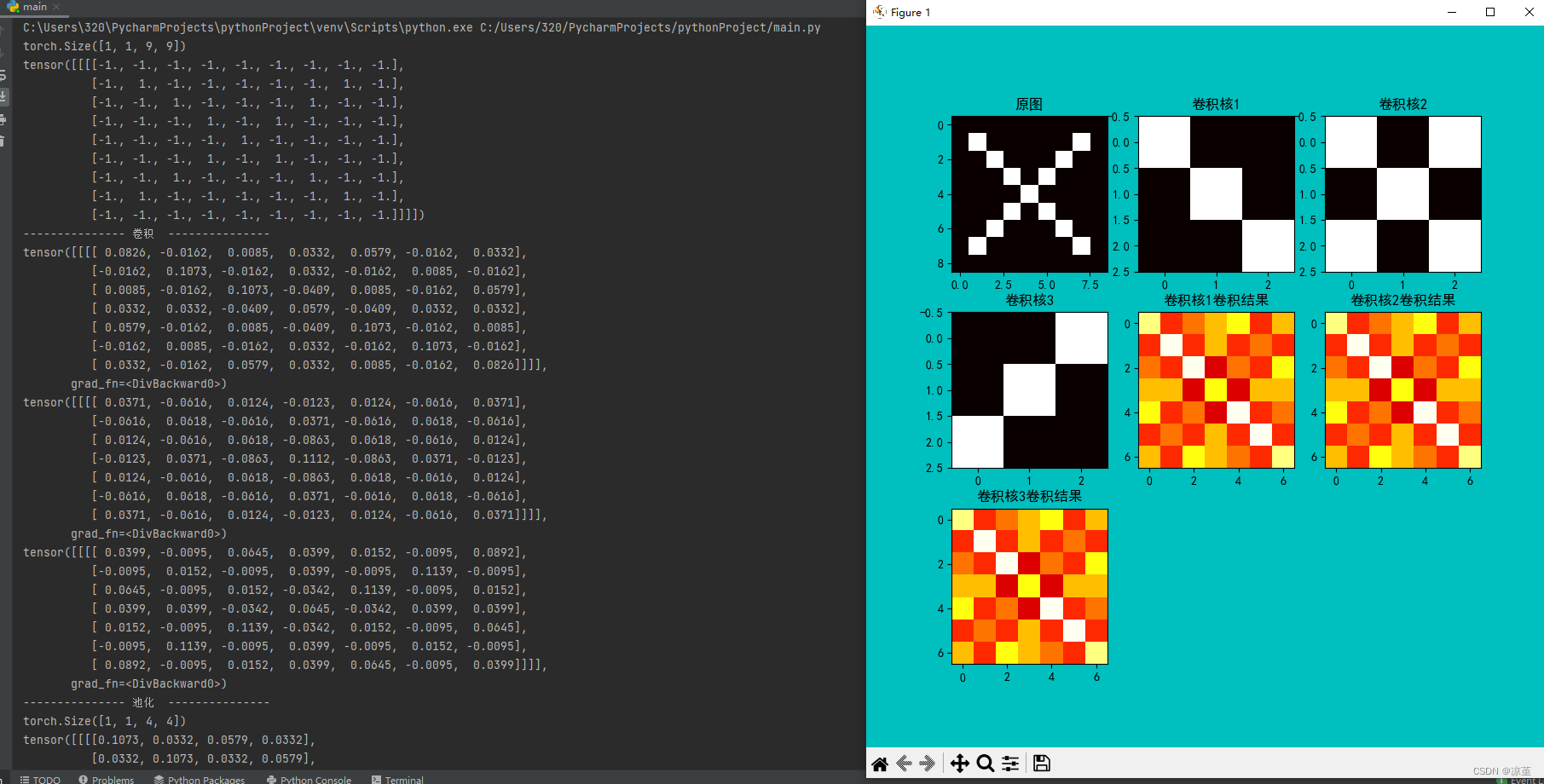
2. Pytorch版本:调用函数实现 卷积-池化-激活
调用框架自带算子实现,对比自定义算子
代码如下:
import torch
import torch.nn as nn
import matplotlib.pyplot as plt

plt.rcParams['font.sans-serif'] = ['SimHei']  # 用来正常显示中文标签
plt.rcParams['axes.unicode_minus'] = False  # 用来正常显示负号 #有中文出现的情况,需要u'内容
x = torch.tensor([[[[-1, -1, -1, -1, -1, -1, -1, -1, -1],
                    [-1, 1, -1, -1, -1, -1, -1, 1, -1],
                    [-1, -1, 1, -1, -1, -1, 1, -1, -1],
                    [-1, -1, -1, 1, -1, 1, -1, -1, -1],
                    [-1, -1, -1, -1, 1, -1, -1, -1, -1],
                    [-1, -1, -1, 1, -1, 1, -1, -1, -1],
                    [-1, -1, 1, -1, -1, -1, 1, -1, -1],
                    [-1, 1, -1, -1, -1, -1, -1, 1, -1],
                    [-1, -1, -1, -1, -1, -1, -1, -1, -1]]]], dtype=torch.float)
print(x.shape)
print(x)
img = x.data.squeeze().numpy()  # 将输出转换为图片的格式
print("--------------- 卷积  ---------------")
conv1 = nn.Conv2d(1, 1, (3, 3), 1)  # in_channel , out_channel , kennel_size , stride
conv1.weight.data = torch.Tensor([[[[1, -1, -1],
                                    [-1, 1, -1],
                                    [-1, -1, 1]]
                                   ]])
img2 = conv1.weight.data.squeeze().numpy()  # 将输出转换为图片的格式
conv2 = nn.Conv2d(1, 1, (3, 3), 1)  # in_channel , out_channel , kennel_size , stride
conv2.weight.data = torch.Tensor([[[[1, -1, 1],
                                    [-1, 1, -1],
                                    [1, -1, 1]]
                                   ]])
img3 = conv2.weight.data.squeeze().numpy()  # 将输出转换为图片的格式
conv3 = nn.Conv2d(1, 1, (3, 3), 1)  # in_channel , out_channel , kennel_size , stride
conv3.weight.data = torch.Tensor([[[[-1, -1, 1],
                                    [-1, 1, -1],
                                    [1, -1, -1]]
                                   ]])
img4 = conv3.weight.data.squeeze().numpy()  # 将输出转换为图片的格式
plt.figure(1, figsize=[50, 50], edgecolor='c', facecolor='c')
plt.subplot(331).set_title('原图')
plt.imshow(img, cmap=plt.cm.hot, vmin=-1, vmax=1)
plt.subplot(332).set_title('卷积核1')
plt.imshow(img2, cmap=plt.cm.hot, vmin=-1, vmax=1)
plt.subplot(333).set_title('卷积核2')
plt.imshow(img3, cmap=plt.cm.hot, vmin=-1, vmax=1)
plt.subplot(334).set_title('卷积核3')
plt.imshow(img4, cmap=plt.cm.hot, vmin=-1, vmax=1)

feature_map1 = conv1(x) / 9
feature_map2 = conv2(x) / 9
feature_map3 = conv3(x) / 9

print(feature_map1 / 9)
print(feature_map2 / 9)
print(feature_map3 / 9)
img5 = feature_map1.data.squeeze().numpy()  # 将输出转换为图片的格式
img6 = feature_map1.data.squeeze().numpy()  # 将输出转换为图片的格式
img7 = feature_map1.data.squeeze().numpy()  # 将输出转换为图片的格式

plt.subplot(335).set_title('卷积核1卷积结果')
plt.imshow(img5, cmap=plt.cm.hot, vmin=-1, vmax=1)
plt.subplot(336).set_title('卷积核2卷积结果')
plt.imshow(img6, cmap=plt.cm.hot, vmin=-1, vmax=1)
plt.subplot(337).set_title('卷积核3卷积结果')
plt.imshow(img7, cmap=plt.cm.hot, vmin=-1, vmax=1)

print("--------------- 池化  ---------------")
max_pool = nn.MaxPool2d(2, padding=0, stride=2)  # Pooling
zeroPad = nn.ZeroPad2d(padding=(0, 1, 0, 1))  # pad 0 , Left Right Up Down

feature_map_pad_0_1 = zeroPad(feature_map1)
feature_pool_1 = max_pool(feature_map_pad_0_1)
feature_map_pad_0_2 = zeroPad(feature_map2)
feature_pool_2 = max_pool(feature_map_pad_0_2)
feature_map_pad_0_3 = zeroPad(feature_map3)
feature_pool_3 = max_pool(feature_map_pad_0_3)

print(feature_pool_1.size())
print(feature_pool_1 / 9)
print(feature_pool_2 / 9)
print(feature_pool_3 / 9)
img = feature_pool_1.data.squeeze().numpy()  # 将输出转换为图片的格式
plt.figure(2, figsize=[50, 50], edgecolor='c', facecolor='c')
plt.subplot(331).set_title('特征图1补零结果')
plt.imshow(feature_map_pad_0_1.data.squeeze().numpy(), cmap=plt.cm.hot, vmin=-1, vmax=1)
plt.subplot(332).set_title('特征图2补零结果')
plt.imshow(feature_map_pad_0_2.data.squeeze().numpy(), cmap=plt.cm.hot, vmin=-1, vmax=1)
plt.subplot(333).set_title('特征图3补零结果')
plt.imshow(feature_map_pad_0_3.data.squeeze().numpy(), cmap=plt.cm.hot, vmin=-1, vmax=1)
plt.subplot(334).set_title('特征图1补零后池化结果')
plt.imshow(feature_pool_1.data.squeeze().numpy(), cmap=plt.cm.hot, vmin=-1, vmax=1)
plt.subplot(335).set_title('特征图2补零后池化结果')
plt.imshow(feature_pool_2.data.squeeze().numpy(), cmap=plt.cm.hot, vmin=-1, vmax=1)
plt.subplot(336).set_title('特征图3补零后池化结果')
plt.imshow(feature_pool_3.data.squeeze().numpy(), cmap=plt.cm.hot, vmin=-1, vmax=1)
print("--------------- 激活  ---------------")
activation_function = nn.ReLU()
feature_relu1 = activation_function(feature_map1)
feature_relu2 = activation_function(feature_map2)
feature_relu3 = activation_function(feature_map3)
print(feature_relu1 / 9)
print(feature_relu2 / 9)
print(feature_relu3 / 9)
plt.subplot(337).set_title('特征图1池化后Relu激活结果')
plt.imshow(feature_relu1.data.squeeze().numpy(), cmap=plt.cm.hot, vmin=-1, vmax=1)
plt.subplot(338).set_title('特征图2池化后Relu激活结果')
plt.imshow(feature_relu2.data.squeeze().numpy(), cmap=plt.cm.hot, vmin=-1, vmax=1)
plt.subplot(339).set_title('特征图3池化后Relu激活结果')
plt.imshow(feature_relu3.data.squeeze().numpy(), cmap=plt.cm.hot, vmin=-1, vmax=1)
plt.show()
运行结果:

二、 基于CNN的XO识别
1. 数据集
QQ群下载
【注】
QQ群内下载的数据集没有分测试集和训练集。
共2000张图片,X、O各1000张。
从X、O文件夹,分别取出150张作为测试集。
文件夹train_data:放置训练集 1700张图片
文件夹test_data: 放置测试集 300张图片
代码如下:
import torch
from torchvision import transforms, datasets
import torch.nn as nn
from torch.utils.data import DataLoader
import torch.optim as optim
import matplotlib.pyplot as plt

transforms = transforms.Compose([
    transforms.ToTensor(),  # 把图片进行归一化,并把数据转换成Tensor类型
    transforms.Grayscale(1)  # 把图片 转为灰度图
])

path_test = r'C:\Users\Administrator\Desktop\test_data'
path = r'C:\Users\Administrator\Desktop\train_data'

data_train = datasets.ImageFolder(path, transform=transforms)
data_test = datasets.ImageFolder(path_test, transform=transforms)

print("size of train_data:", len(data_train))
print("size of test_data:", len(data_test))

data_loader = DataLoader(data_train, batch_size=64, shuffle=True)
data_loader_test = DataLoader(data_test, batch_size=64, shuffle=True)

for i, data in enumerate(data_loader):
    images, labels = data
    print(images.shape)
    print(labels.shape)
    break

for i, data in enumerate(data_loader_test):
    images, labels = data
    print(images.shape)
    print(labels.shape)
    break
运行结果:

2. 构建模型
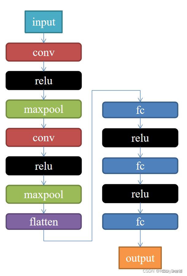
代码如下:
class Net(nn.Module):
    def __init__(self):
        super(Net, self).__init__()
        self.conv1 = nn.Conv2d(1, 9, 3)
        self.maxpool = nn.MaxPool2d(2, 2)
        self.conv2 = nn.Conv2d(9, 5, 3)

        self.relu = nn.ReLU()
        self.fc1 = nn.Linear(27 * 27 * 5, 1200)
        self.fc2 = nn.Linear(1200, 64)
        self.fc3 = nn.Linear(64, 2)

    def forward(self, x):
        x = self.maxpool(self.relu(self.conv1(x)))
        x = self.maxpool(self.relu(self.conv2(x)))
        x = x.view(-1, 27 * 27 * 5)
        x = self.relu(self.fc1(x))
        x = self.relu(self.fc2(x))
        x = self.fc3(x)
        return x
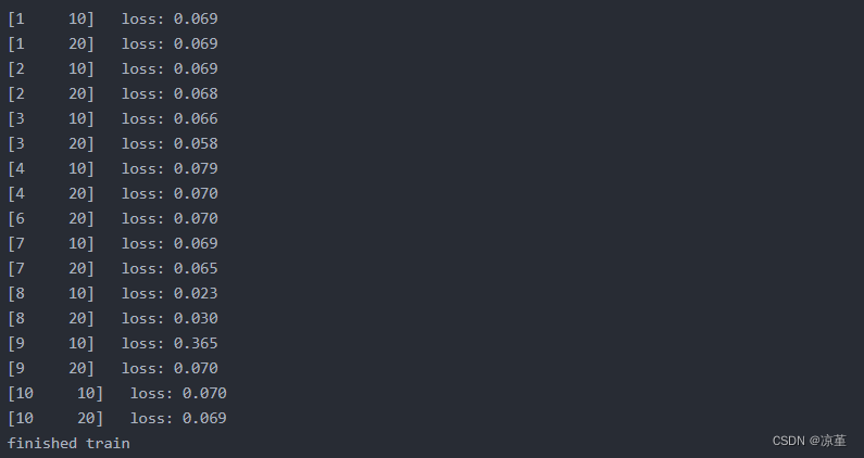
3.训练模型
代码如下:
model = Net()

criterion = torch.nn.CrossEntropyLoss()  # 损失函数 交叉熵损失函数
optimizer = optim.SGD(model.parameters(), lr=0.1)  # 优化函数:随机梯度下降

epochs = 10
for epoch in range(epochs):
    running_loss = 0.0
    for i, data in enumerate(data_loader):
        images, label = data
        out = model(images)
        loss = criterion(out, label)

        optimizer.zero_grad()
        loss.backward()
        optimizer.step()

        running_loss += loss.item()
        if (i + 1) % 10 == 0:
            print('[%d  %5d]   loss: %.3f' % (epoch + 1, i + 1, running_loss / 100))
            running_loss = 0.0

print('finished train')

# 保存模型
torch.save(model, 'model_name.pth')  # 保存的是模型, 不止是w和b权重值
运行结果:
4、测试训练好的模型
代码如下:
# 读取模型
model_load = torch.load('model_name.pth')
# 读取一张图片 images[0],测试
print("labels[0] truth:\t", labels[0])
x = images[0]
x = x.reshape([1, x.shape[0], x.shape[1], x.shape[2]])
predicted = torch.max(model_load(x), 1)
print("labels[0] predict:\t", predicted.indices)

img = images[0].data.squeeze().numpy()  # 将输出转换为图片的格式
plt.imshow(img, cmap='gray')
plt.show()
运行结果:


5、计算模型的准确率
代码如下:
# 读取模型
model_load = torch.load('model_name.pth')

correct = 0
total = 0
with torch.no_grad():  # 进行评测的时候网络不更新梯度
    for data in data_loader_test:  # 读取测试集
        images, labels = data
        outputs = model_load(images)
        _, predicted = torch.max(outputs.data, 1)  # 取出 最大值的索引 作为 分类结果
        total += labels.size(0)  # labels 的长度
        correct += (predicted == labels).sum().item()  # 预测正确的数目
print('Accuracy of the network on the  test images: %f %%' % (100. * correct / total))
运行结果:

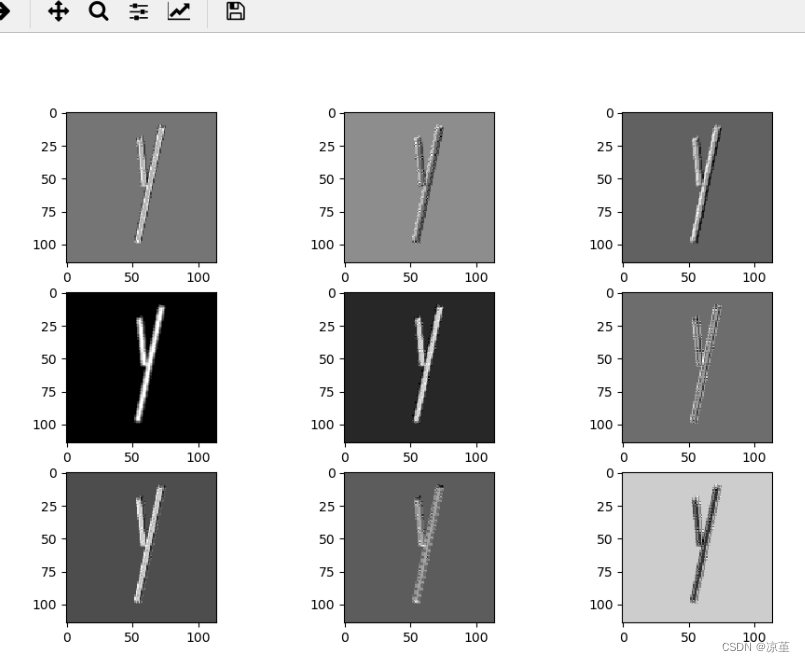
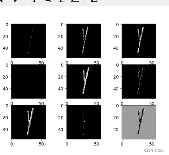
6、查看训练好的模型特征图
代码如下:
import torch
import matplotlib.pyplot as plt
import numpy as np
from torchvision import transforms, datasets
import torch.nn as nn
from torch.utils.data import DataLoader

# 定义图像预处理过程
transforms = transforms.Compose([
    transforms.ToTensor(),  # 把图片进行归一化,并把数据转换成Tensor类型
    transforms.Grayscale(1)  # 把图片 转为灰度图
])
path = r'路径'
data_train = datasets.ImageFolder(path, transform=transforms)
data_loader = DataLoader(data_train, batch_size=64, shuffle=True)
for i, data in enumerate(data_loader):
    images, labels = data
    print(images.shape)
    print(labels.shape)
    break


class Net(nn.Module):
    def __init__(self):
        super(Net, self).__init__()
        self.conv1 = nn.Conv2d(1, 9, 3)  # in_channel , out_channel , kennel_size , stride
        self.maxpool = nn.MaxPool2d(2, 2)
        self.conv2 = nn.Conv2d(9, 5, 3)  # in_channel , out_channel , kennel_size , stride

        self.relu = nn.ReLU()
        self.fc1 = nn.Linear(27 * 27 * 5, 1200)  # full connect 1
        self.fc2 = nn.Linear(1200, 64)  # full connect 2
        self.fc3 = nn.Linear(64, 2)  # full connect 3

    def forward(self, x):
        outputs = []
        x = self.conv1(x)
        outputs.append(x)
        x = self.relu(x)
        outputs.append(x)
        x = self.maxpool(x)
        outputs.append(x)
        x = self.conv2(x)
        x = self.relu(x)
        x = self.maxpool(x)
        x = x.view(-1, 27 * 27 * 5)
        x = self.relu(self.fc1(x))
        x = self.relu(self.fc2(x))
        x = self.fc3(x)
        return outputs

# load model weights加载预训练权重
model_weight_path = "model_name.pth"
model1 = torch.load(model_weight_path)

# 打印出模型的结构
print(model1)
x = images[0]
x = x.reshape([1, x.shape[0], x.shape[1], x.shape[2]])
# forward正向传播过程
out_put = model1(x)
for feature_map in out_put:
    im = np.squeeze(feature_map.detach().numpy())
    im = np.transpose(im, [1, 2, 0])
    print(im.shape)

    plt.figure()
    for i in range(9):
        ax = plt.subplot(3, 3, i + 1)
        plt.imshow(im[:, :, i], cmap='gray')
    plt.show()
运行结果:

第一轮
第二轮

第三轮
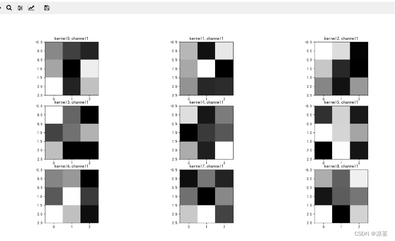
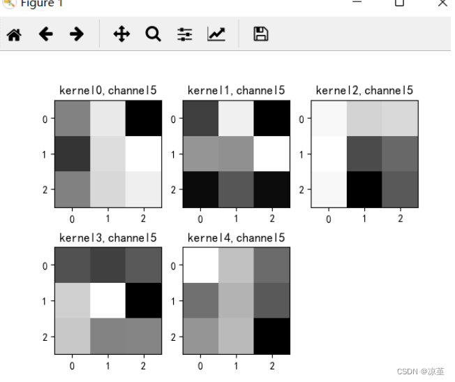
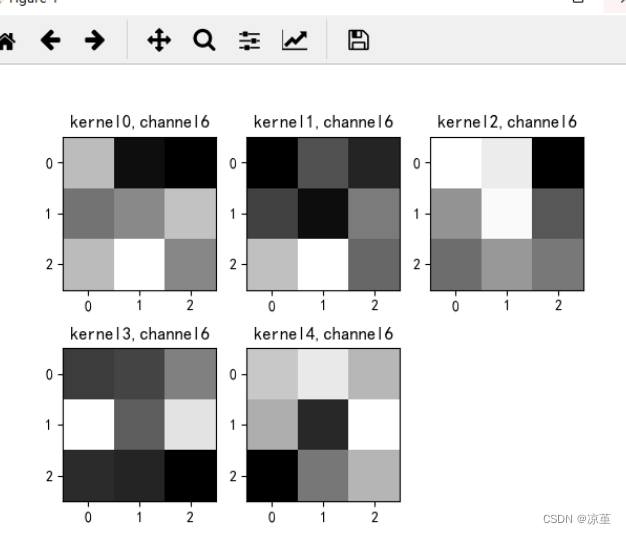
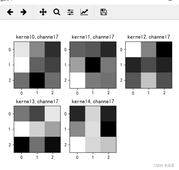
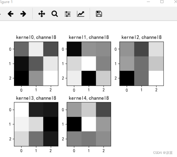
7、查看训练好的卷积核
代码如下:
import torch
import matplotlib.pyplot as plt
import numpy as np
from PIL import Image
from torchvision import transforms, datasets
import torch.nn as nn
from torch.utils.data import DataLoader
plt.rcParams['font.sans-serif'] = ['SimHei'] # 用来正常显示中文标签
plt.rcParams['axes.unicode_minus'] = False # 用来正常显示负号 #有中文出现的情况,需要u'内容
# 定义图像预处理过程(要与网络模型训练过程中的预处理过程一致)
transforms = transforms.Compose([
transforms.ToTensor(), # 把图片进行归一化,并把数据转换成Tensor类型
transforms.Grayscale(1) # 把图片 转为灰度图
])
path = r'D:\project\DL\training_data_sm'
data_train = datasets.ImageFolder(path, transform=transforms)
data_loader = DataLoader(data_train, batch_size=64, shuffle=True)
for i, data in enumerate(data_loader):
images, labels = data
break
class Net(nn.Module):
def __init__(self):
super(Net, self).__init__()
self.conv1 = nn.Conv2d(1, 9, 3) # in_channel , out_channel , kennel_size , stride
self.maxpool = nn.MaxPool2d(2, 2)
self.conv2 = nn.Conv2d(9, 5, 3) # in_channel , out_channel , kennel_size , stride
self.relu = nn.ReLU()
self.fc1 = nn.Linear(27 * 27 * 5, 1200) # full connect 1
self.fc2 = nn.Linear(1200, 64) # full connect 2
self.fc3 = nn.Linear(64, 2) # full connect 3
def forward(self, x):
outputs = []
x = self.maxpool(self.relu(self.conv1(x)))
# outputs.append(x)
x = self.maxpool(self.relu(self.conv2(x)))
outputs.append(x)
x = x.view(-1, 27 * 27 * 5)
x = self.relu(self.fc1(x))
x = self.relu(self.fc2(x))
x = self.fc3(x)
return outputs
# create model
model1 = Net()
# load model weights加载预训练权重
model_weight_path = "model_name1.pth"
model1.load_state_dict(torch.load(model_weight_path))
x = images[0]
x = x.reshape([1, x.shape[0], x.shape[1], x.shape[2]])
# forward正向传播过程
out_put = model1(x)
weights_keys = model1.state_dict().keys()
for key in weights_keys:
print("key :", key)
# 卷积核通道排列顺序 [kernel_number, kernel_channel, kernel_height, kernel_width]
if key == "conv1.weight":
weight_t = model1.state_dict()[key].numpy()
print("weight_t.shape", weight_t.shape)
k = weight_t[:, 0, :, :] # 获取第一个卷积核的信息参数
# show 9 kernel ,1 channel
plt.figure()
for i in range(9):
ax = plt.subplot(3, 3, i + 1) # 参数意义:3:图片绘制行数,5:绘制图片列数,i+1:图的索引
plt.imshow(k[i, :, :], cmap='gray')
title_name = 'kernel' + str(i) + ',channel1'
plt.title(title_name)
plt.show()
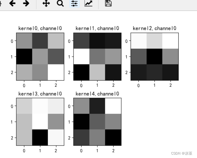
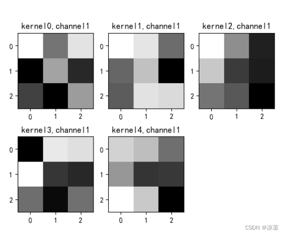
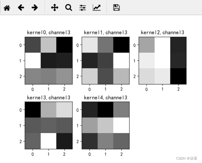
if key == "conv2.weight":
weight_t = model1.state_dict()[key].numpy()
print("weight_t.shape", weight_t.shape)
k = weight_t[:, :, :, :] # 获取第一个卷积核的信息参数
print(k.shape)
print(k)
plt.figure()
for c in range(9):
channel = k[:, c, :, :]
for i in range(5):
ax = plt.subplot(2, 3, i + 1) # 参数意义:3:图片绘制行数,5:绘制图片列数,i+1:图的索引
plt.imshow(channel[i, :, :], cmap='gray')
title_name = 'kernel' + str(i) + ',channel' + str(c)
plt.title(title_name)
plt.show()
运行结果:
key : conv1.weight
weight_t.shape (9, 1, 3, 3)
key : conv1.bias
key : conv2.weight
weight_t.shape (5, 9, 3, 3)
(5, 9, 3, 3)
[[[[ 2.13337447e-02 -4.66020554e-02  5.69471493e-02]
   [-9.50448960e-02  2.72415876e-02 -2.67830752e-02]
   [ 4.33921367e-02  1.58538613e-02  1.07408538e-01]]

  [[ 5.92437796e-02 -2.98182946e-02  4.08032201e-02]
   [-1.04227282e-01  4.49235813e-04 -7.80264363e-02]
   [-6.20211102e-02 -1.03927836e-01 -4.45224531e-03]]

  [[-8.12148899e-02 -3.29005569e-02 -1.01220481e-01]
   [-5.81114963e-02  8.76028463e-02  2.85280328e-02]
   [ 6.18191846e-02  1.11722171e-01  1.05508761e-02]]

  [[ 2.56348290e-02  8.95467028e-02 -1.04550337e-02]
   [ 1.20045662e-01  3.91172059e-03  6.04839716e-03]
   [ 5.81633002e-02  5.49804084e-02  6.52925819e-02]]

  [[-1.03181293e-02 -9.07509103e-02 -5.63313253e-03]
   [ 7.76769295e-02  8.91671702e-03 -5.17778061e-02]
   [ 1.84927054e-03 -3.96537296e-02 -3.72357517e-02]]

  [[ 2.83653126e-03  9.17217806e-02 -1.08959302e-01]
   [-6.36169314e-02  8.10930431e-02  1.11177579e-01]
   [ 2.64830631e-03  7.71028176e-02  9.69813466e-02]]

  [[ 5.95637821e-02 -6.03413619e-02 -7.06231743e-02]
   [ 8.84121284e-03  2.43839268e-02  6.31544441e-02]
   [ 5.85174784e-02  1.05725035e-01  2.27449443e-02]]

  [[ 8.67228359e-02  1.13745630e-02 -5.97287230e-02]
   [ 1.06772520e-01 -1.83142200e-02 -4.38390411e-02]
   [-7.93279801e-03 -9.62066352e-02 -9.74365976e-03]]

  [[-2.83114128e-02  6.16717227e-02 -4.58590016e-02]
   [-8.79971832e-02 -3.77490371e-02  5.77585809e-02]
   [-9.76629704e-02  1.47018349e-03  7.31262490e-02]]]


 [[[-4.13246527e-02 -8.10668841e-02 -7.33139515e-02]
   [ 1.07044421e-01 -1.22925197e-03  2.60232706e-02]
   [-9.28884670e-02  5.91737926e-02 -7.68024623e-02]]

  [[ 1.00566290e-01  7.92008340e-02 -1.99213047e-02]
   [-2.53674462e-02  4.92495708e-02 -1.09196201e-01]
   [-3.30992639e-02  7.65849128e-02  6.94890991e-02]]

  [[ 8.79835114e-02  7.17155784e-02  9.48633347e-03]
   [-8.04083794e-02 -3.33686396e-02 -1.03847809e-01]
   [-9.38878879e-02 -2.61832345e-02  2.34493092e-02]]

  [[ 7.49496520e-02 -6.58766134e-03 -9.02236775e-02]
   [-6.38174117e-02 -4.38476242e-02  9.28886160e-02]
   [ 6.03966303e-02 -3.48509438e-02  4.21662889e-02]]

  [[-1.07795596e-01 -4.21107486e-02  1.35774277e-02]
   [-5.69701381e-02 -2.53783017e-02 -7.26861283e-02]
   [ 6.95042908e-02 -1.94982961e-02 -1.04479250e-02]]

  [[-5.16788289e-03  9.92982760e-02 -4.29186560e-02]
   [ 4.52080965e-02  4.26085629e-02  1.08374067e-01]
   [-3.60247716e-02  7.95567874e-03 -3.53158526e-02]]

  [[-9.03374851e-02 -4.17616405e-02 -6.89267069e-02]
   [-5.10569401e-02 -8.26060697e-02 -1.68968644e-02]
   [ 2.40772069e-02  6.16443269e-02 -2.88375039e-02]]

  [[-2.65944675e-02 -3.34033631e-02 -6.38400391e-02]
   [ 1.19640520e-02 -8.90198499e-02 -1.31003242e-02]
   [ 7.28889033e-02 -1.08855562e-02 -1.69340577e-02]]

  [[-8.96208510e-02  7.17032515e-03  2.98084784e-03]
   [ 5.63147925e-02  8.42373669e-02 -3.07463785e-03]
   [ 7.20602646e-02 -9.59975421e-02  4.89495136e-02]]]


 [[[ 8.73266608e-02  6.21295087e-02  9.09073725e-02]
   [-3.66917998e-02 -1.06961414e-01  2.33189273e-03]
   [-8.58709216e-02 -7.66173601e-02 -8.92223716e-02]]

  [[ 1.42468750e-01  4.55042571e-02 -4.87571731e-02]
   [ 9.50629860e-02 -2.55978256e-02 -5.17828055e-02]
   [ 2.28720512e-02 -4.18525684e-04 -7.64779896e-02]]

  [[ 2.13523954e-01  2.11181626e-01  6.31329343e-02]
   [ 2.93317258e-01  1.79045513e-01  9.32165161e-02]
   [ 1.64305896e-01  1.73994735e-01 -2.24261004e-02]]

  [[ 1.01647288e-01  1.82940543e-01 -1.32072493e-02]
   [ 1.67549968e-01  1.83086529e-01 -1.15432255e-02]
   [ 1.49951175e-01  1.63617715e-01 -4.67457622e-02]]

  [[ 9.69711915e-02  2.44501099e-01  3.42077821e-01]
   [ 2.81096280e-01  2.47293875e-01  3.15020204e-01]
   [ 2.30779156e-01  2.49916524e-01  1.14863127e-01]]

  [[ 1.22386098e-01  9.09488872e-02  9.59159583e-02]
   [ 1.28422126e-01 -2.54476443e-02 -1.23610243e-03]
   [ 1.21951476e-01 -9.00956392e-02 -1.30032878e-02]]

  [[ 2.70890594e-01  2.51383096e-01  1.19242668e-02]
   [ 1.61680534e-01  2.65115023e-01  1.00206561e-01]
   [ 1.22219384e-01  1.66553617e-01  1.33594766e-01]]

  [[ 1.26680538e-01  2.05860939e-02 -8.89521614e-02]
   [-5.75781688e-02 -2.44606063e-02 -5.95157966e-02]
   [-1.51281776e-02  7.65277594e-02 -1.97108556e-02]]

  [[-1.56779736e-02 -8.56565610e-02  5.39452508e-02]
   [-5.56658115e-03 -4.77824248e-02  3.06996740e-02]
   [-1.49981990e-01 -4.82937209e-02  8.32402334e-02]]]


 [[[ 7.32601061e-02  1.04371667e-01  9.47857574e-02]
   [ 6.02787100e-02  1.06775448e-01  2.70277727e-02]
   [ 6.06970973e-02 -8.14046264e-02  1.01076826e-01]]

  [[-4.07370068e-02  1.32704556e-01  1.24955118e-01]
   [ 1.49428457e-01 -1.35628521e-04 -1.06292712e-02]
   [ 4.10106331e-02 -3.27576511e-02  4.31486629e-02]]

  [[ 1.47851288e-01  7.37611949e-02 -8.00638052e-04]
   [ 5.49609214e-02  5.39804809e-02  1.64051205e-01]
   [ 1.86090365e-01  7.10770637e-02  1.11168213e-01]]

  [[ 3.99321988e-02  1.22020051e-01  1.42244220e-01]
   [ 8.14780816e-02  8.58630985e-02  8.22043419e-02]
   [ 8.61948952e-02  1.58883244e-01  5.22515438e-02]]

  [[-6.07095752e-03  6.35409951e-02  1.17611088e-01]
   [ 1.33611187e-01  1.53549671e-01  2.12974072e-01]
   [ 1.88580588e-01  2.44575635e-01  1.57943800e-01]]

  [[-3.28077078e-02 -4.73249964e-02 -2.52703018e-02]
   [ 7.68502131e-02  1.17673844e-01 -1.02793567e-01]
   [ 6.95649087e-02  1.08037842e-02  1.20138116e-02]]

  [[ 6.12324141e-02  6.74496293e-02  1.17424197e-01]
   [ 2.23221451e-01  8.87446627e-02  2.00333238e-01]
   [ 4.64970693e-02  4.10990007e-02  9.99209099e-03]]

  [[ 2.60900036e-02 -9.70500242e-03  1.03694111e-01]
   [ 1.20320909e-01  8.78464282e-02  5.51295951e-02]
   [-5.68686947e-02  2.27155127e-02 -4.86865342e-02]]

  [[ 7.43962973e-02 -1.07168131e-01 -1.14755601e-01]
   [ 6.45004362e-02  4.48054969e-02 -1.34845525e-01]
   [ 4.38693687e-02 -4.12172489e-02 -1.13492347e-01]]]


 [[[ 9.75735486e-03 -8.00553411e-02  9.98245627e-02]
   [-1.03557631e-01 -3.00987791e-02  2.47929199e-03]
   [-5.84659129e-02 -3.11498647e-03 -1.05383299e-01]]

  [[ 8.14179480e-02  6.47853762e-02 -1.35293370e-03]
   [ 3.17397229e-02 -4.96356338e-02 -4.67157252e-02]
   [ 1.18946128e-01  7.36141875e-02 -9.43131968e-02]]

  [[ 4.32302430e-02  8.00670218e-03  1.30381286e-01]
   [ 1.58645473e-02  8.79430696e-02  7.13290200e-02]
   [-9.26138014e-02  1.08460955e-01  4.07457128e-02]]

  [[-5.52411787e-02 -7.14086965e-02 -1.40719339e-02]
   [ 1.10834430e-03  1.85057782e-02  4.45450768e-02]
   [-4.88245822e-02 -1.27766682e-02 -2.52490900e-02]]

  [[-3.18568014e-02 -7.60855377e-02 -4.60483227e-03]
   [ 1.11823879e-01 -9.02110152e-03  1.35904774e-01]
   [-5.47109060e-02  9.24533792e-03 -5.56159299e-03]]

  [[ 9.89506766e-02  5.30992337e-02 -1.05850836e-02]
   [-7.10224826e-03  4.21758369e-02 -2.33692788e-02]
   [ 2.01377794e-02  4.78765368e-02 -8.98735225e-02]]

  [[ 8.93814713e-02  1.14521869e-01  7.65397772e-02]
   [ 6.96704984e-02 -3.08779012e-02  1.31388307e-01]
   [-6.19704947e-02  2.86297128e-02  7.49430656e-02]]

  [[-8.53083134e-02  2.83263866e-02 -8.79642963e-02]
   [-2.06125565e-02  3.40545662e-02 -1.09950185e-01]
   [ 5.58296703e-02  2.96729505e-02  1.78528689e-02]]

  [[ 2.82099899e-02  5.61815053e-02 -2.08272506e-02]
   [-6.34855852e-02  8.60610232e-02  2.67249420e-02]
   [ 1.40091237e-02  7.67472852e-03  1.93426870e-02]]]]
   key : conv2.bias
key : fc1.weight
key : fc1.bias
key : fc2.weight
key : fc2.bias
key : fc3.weight
key : fc3.bias
第一轮
第二轮
8、训练模型源代码
代码如下:
import torch
from torchvision import transforms, datasets
import torch.nn as nn
from torch.utils.data import DataLoader
import matplotlib.pyplot as plt
import torch.optim as optim

transforms = transforms.Compose([
    transforms.ToTensor(),  # 把图片进行归一化,并把数据转换成Tensor类型
    transforms.Grayscale(1)  # 把图片 转为灰度图
])

path = r'train_data'
path_test = r'test_data'

data_train = datasets.ImageFolder(path, transform=transforms)
data_test = datasets.ImageFolder(path_test, transform=transforms)

print("size of train_data:", len(data_train))
print("size of test_data:", len(data_test))

data_loader = DataLoader(data_train, batch_size=64, shuffle=True)
data_loader_test = DataLoader(data_test, batch_size=64, shuffle=True)

for i, data in enumerate(data_loader):
    images, labels = data
    print(images.shape)
    print(labels.shape)
    break

for i, data in enumerate(data_loader_test):
    images, labels = data
    print(images.shape)
    print(labels.shape)
    break


class Net(nn.Module):
    def __init__(self):
        super(Net, self).__init__()
        self.conv1 = nn.Conv2d(1, 9, 3)  # in_channel , out_channel , kennel_size , stride
        self.maxpool = nn.MaxPool2d(2, 2)
        self.conv2 = nn.Conv2d(9, 5, 3)  # in_channel , out_channel , kennel_size , stride

        self.relu = nn.ReLU()
        self.fc1 = nn.Linear(27 * 27 * 5, 1200)  # full connect 1
        self.fc2 = nn.Linear(1200, 64)  # full connect 2
        self.fc3 = nn.Linear(64, 2)  # full connect 3

    def forward(self, x):
        x = self.maxpool(self.relu(self.conv1(x)))
        x = self.maxpool(self.relu(self.conv2(x)))
        x = x.view(-1, 27 * 27 * 5)
        x = self.relu(self.fc1(x))
        x = self.relu(self.fc2(x))
        x = self.fc3(x)
        return x


model = Net()

criterion = torch.nn.CrossEntropyLoss()  # 损失函数 交叉熵损失函数
optimizer = optim.SGD(model.parameters(), lr=0.1)  # 优化函数:随机梯度下降

epochs = 10
for epoch in range(epochs):
    running_loss = 0.0
    for i, data in enumerate(data_loader):
        images, label = data
        out = model(images)
        loss = criterion(out, label)

        optimizer.zero_grad()
        loss.backward()
        optimizer.step()

        running_loss += loss.item()
        if (i + 1) % 10 == 0:
            print('[%d  %5d]   loss: %.3f' % (epoch + 1, i + 1, running_loss / 100))
            running_loss = 0.0

print('finished train')

# 保存模型 torch.save(model.state_dict(), model_path)
torch.save(model.state_dict(), 'model_name.pth')  # 保存的是模型, 不止是w和b权重值


# 读取一张图片 images[0],测试
print("labels[0] truth:\t", labels[0])
x = images[0]
x =torch.unsqueeze(x, dim=0)
predicted = torch.max(model(x), 1)
print("labels[0] predict:\t", predicted.indices)

img = images[0].data.squeeze().numpy()  # 将输出转换为图片的格式
plt.imshow(img, cmap='gray')
plt.show()
9、测试源代码
代码如下:
import torch
from torchvision import transforms, datasets
import torch.nn as nn
from torch.utils.data import DataLoader
import matplotlib.pyplot as plt
import torch.optim as optim

transforms = transforms.Compose([
    transforms.ToTensor(),  # 把图片进行归一化,并把数据转换成Tensor类型
    transforms.Grayscale(1)  # 把图片 转为灰度图
])

path = r'train_data'
path_test = r'test_data'

data_train = datasets.ImageFolder(path, transform=transforms)
data_test = datasets.ImageFolder(path_test, transform=transforms)

print("size of train_data:", len(data_train))
print("size of test_data:", len(data_test))

data_loader = DataLoader(data_train, batch_size=64, shuffle=True)
data_loader_test = DataLoader(data_test, batch_size=64, shuffle=True)
print(len(data_loader))
print(len(data_loader_test))


class Net(nn.Module):
    def __init__(self):
        super(Net, self).__init__()
        self.conv1 = nn.Conv2d(1, 9, 3)  # in_channel , out_channel , kennel_size , stride
        self.maxpool = nn.MaxPool2d(2, 2)
        self.conv2 = nn.Conv2d(9, 5, 3)  # in_channel , out_channel , kennel_size , stride

        self.relu = nn.ReLU()
        self.fc1 = nn.Linear(27 * 27 * 5, 1200)  # full connect 1
        self.fc2 = nn.Linear(1200, 64)  # full connect 2
        self.fc3 = nn.Linear(64, 2)  # full connect 3

    def forward(self, x):
        x = self.maxpool(self.relu(self.conv1(x)))
        x = self.maxpool(self.relu(self.conv2(x)))
        x = x.view(-1, 27 * 27 * 5)
        x = self.relu(self.fc1(x))
        x = self.relu(self.fc2(x))
        x = self.fc3(x)
        return x


# 读取模型
model = Net()
model.load_state_dict(torch.load('model_name.pth', map_location='cpu'))  # 导入网络的参数

# model_load = torch.load('model_name1.pth')
# https://blog.csdn.net/qq_41360787/article/details/104332706

correct = 0
total = 0
with torch.no_grad():  # 进行评测的时候网络不更新梯度
    for data in data_loader_test:  # 读取测试集
        images, labels = data
        outputs = model(images)
        _, predicted = torch.max(outputs.data, 1)  # 取出 最大值的索引 作为 分类结果
        total += labels.size(0)  # labels 的长度
        correct += (predicted == labels).sum().item()  # 预测正确的数目
print('Accuracy of the network on the  test images: %f %%' % (100. * correct / total))

#  "_," 的解释 https://blog.csdn.net/weixin_48249563/article/details/111387501
总结
心得体会
这次作业以实践为主,实现了简单的图片数据集的识别,中间保存提取了训练过程,也进行了可视化,训练过程很清楚,便于理解,也更加清楚图片卷积后的变化。其中第二部分作业主要是基于Pytorch搭建简单的卷积网络来实现XO识别,重点是理解卷积过程中的卷积核、特征图的由来以及参数的设置。
参考链接
【2021-2022 春学期】人工智能-作业5:卷积-池化-激活_HBU_David的博客-CSDN博客
【2021-2022 春学期】人工智能-作业6:CNN实现XO识别_HBU_David的博客-CSDN博客


 692
692


 被折叠的 条评论
为什么被折叠?
被折叠的 条评论
为什么被折叠?
 到【灌水乐园】发言


