


✅作者简介:热爱科研的Matlab仿真开发者,修心和技术同步精进,
代码获取、论文复现及科研仿真合作可私信。
🍎个人主页:Matlab科研工作室
🍊个人信条:格物致知。
更多Matlab完整代码及仿真定制内容点击👇
🔥 内容介绍
引力波是爱因斯坦广义相对论的预言,它是由于极端天体运动而产生的时空波动。2015年,引力波首次被直接探测到,这一发现被认为是物理学领域的重大突破。随着引力波探测技术的不断进步,我们现在能够以前所未有的精度和频率探测到引力波信号。然而,引力波数据的分析和重复性是引力波研究中的一个重要议题。
引力波数据的可重复性意味着不同的研究团队在不同的时间和地点能够得到相似的结果。这一特性对于验证和确认引力波探测结果的科学意义至关重要。在引力波研究中,数据的可重复性可以通过多种方式来保证。
首先,数据采集和处理的标准化是保证引力波数据可重复性的关键。引力波探测器的运行和数据采集需要严格遵守一系列标准和规范,以确保数据的准确性和可比性。同时,数据处理和分析的流程也需要进行标准化,以确保不同团队在处理数据时能够得到相似的结果。
其次,开放数据和开放源代码是保证引力波数据可重复性的重要手段。引力波研究中的数据和代码应当尽可能地对外开放,以便其他研究团队能够验证和重复先前的研究结果。开放数据和开放源代码也能够促进引力波研究领域的合作和交流,有助于推动整个领域的发展。
此外,数据分析的透明度和可复现性也是保证引力波数据可重复性的重要因素。研究团队应当清晰地记录数据分析的过程和方法,并在研究成果中提供足够的信息,以便其他团队能够按照相同的方法重复实验。同时,科学期刊和学术出版机构也应当鼓励研究团队在发表研究成果时提供充分的数据和方法细节,以促进数据的可重复性。
总的来说,引力波数据的可重复性是引力波研究中的一个重要问题。通过标准化数据采集和处理流程、开放数据和开放源代码、以及提高数据分析的透明度和可复现性,我们能够保证引力波数据的可重复性,从而验证和确认引力波探测的结果,推动引力波研究领域的发展。希望未来引力波研究能够在数据可重复性方面取得更多的进展,为我们揭示宇宙的奥秘。
📣 部分代码
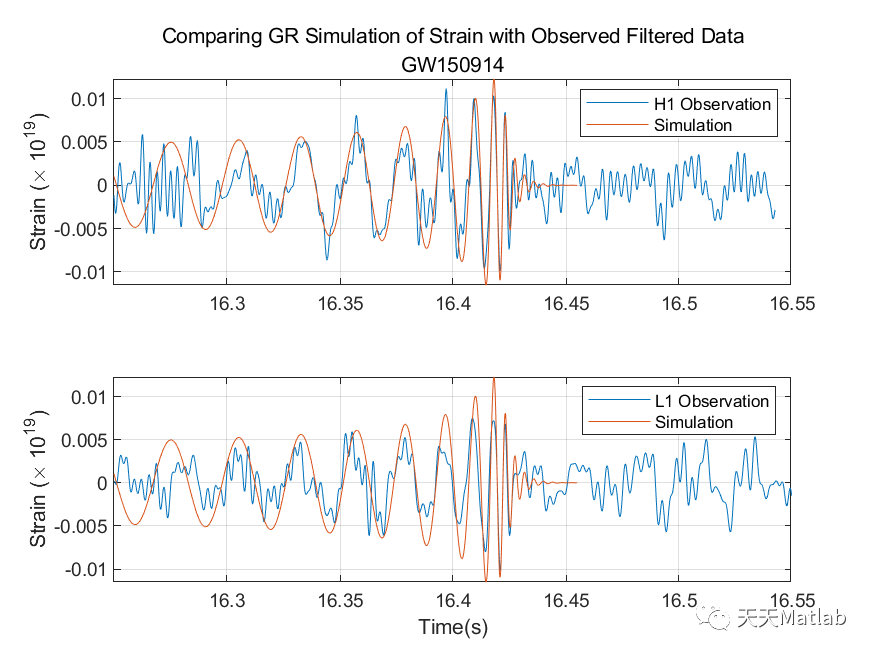
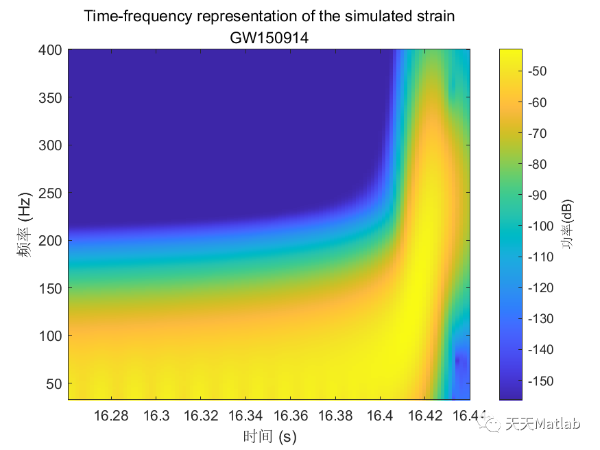
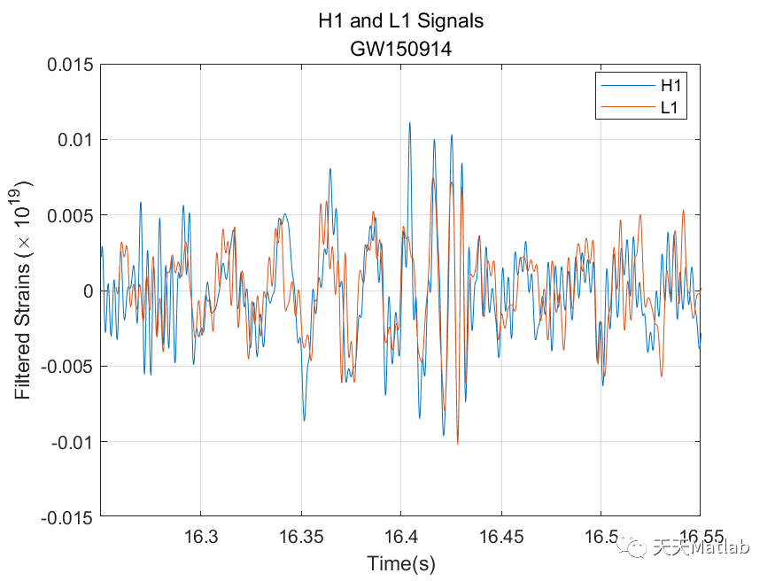
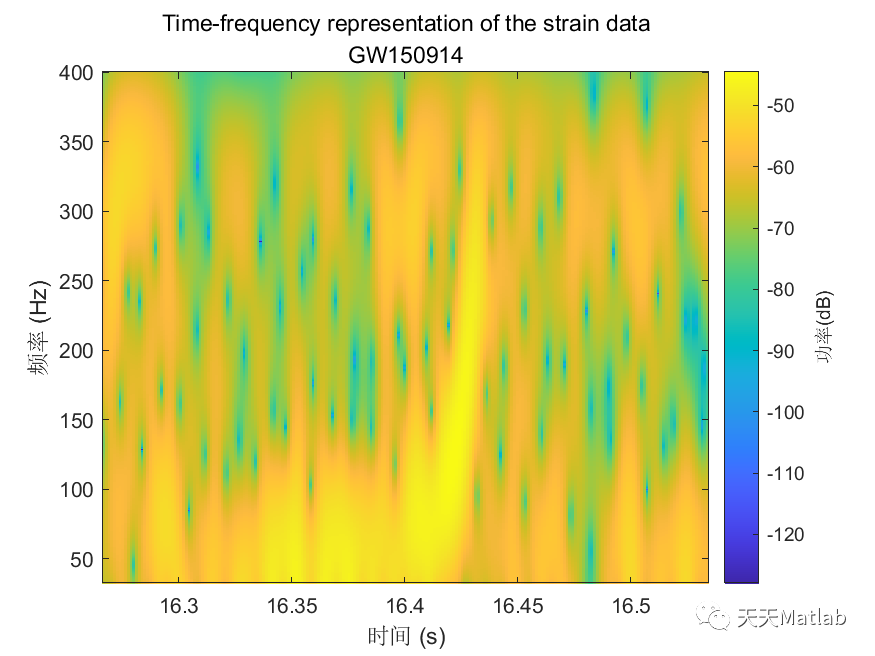
%% Gravitational Wave Data Explorer%% Introduction% *Public Data:* Many public databases have been created for the purposes of% making data freely accessible to the scientific community. A best practice is% to assign a unique identifier to a dataset, so that it is discoverable. A common% form of a unique identifier is a <https://en.wikipedia.org/wiki/Digital_object_identifier% Digital Object Identifier or DOI> which points to the data.%% *Access Public Data:* To access and process public data, you can use several% routes.% * Download data files to your local machine and work with them in MATLAB.% * Access data directly via an API. MATLAB's <https://www.mathworks.com/help/matlab/ref/webread.html?searchHighlight=webread&s_tid=srchtitle_webread_1% |webread|> function reads the RESTful API used by many portals.% * If the portal offers only Python bindings, <https://www.mathworks.com/help/matlab/call-python-libraries.html% call Python from MATLAB>.% *Data formats:* MATLAB supports a wide range of data formats% * There are a wide range of scientific data formats that can be <https://www.mathworks.com/help/matlab/scientific-data.html% natively read in MATLAB>. They include NetCDF and HDF5 as well as more specialized% data formats.% * In addition, MATLAB contains <https://www.mathworks.com/help/matlab/ref/fitsread.html% built-in functions> to read data in specific data formats often used in physics% workflows.% * Sometimes data import functions may be <https://www.mathworks.com/matlabcentral/fileexchange/?category%5B%5D=support%2Fsciences1689.support%2Fphysics1260&q=data+read% written by the community>, and published on the MATLAB <https://www.mathworks.com/matlabcentral/fileexchange/% File Exchange> - a portal for community contributions in MATLAB. All community% contributions are covered by open source licenses, which means they can be re-used,% modified or added to. Exact terms and conditions depend on the licenses used% by the author.% * An example is the code used in this tutorial for strain data exploration% and post-processing which follows this <https://de.mathworks.com/matlabcentral/fileexchange/108859-gravitationalwavedataexplorer?tab=example&focused=% community contribution>. In compliance with the Open Source License used for% this code, the terms of the license are reprinted here.% Copyright (c) 2022, Duncan Carlsmith All rights reserved. Redistribution and% use in source and binary forms, with or without modification, are permitted% provided that the following conditions are met:%% |* Redistributions of source code must retain the above copyright notice,% this list of conditions and the following disclaimer.|%% |* Redistributions in binary form must reproduce the above copyright notice,% this list of conditions and the following disclaimer in the documentation and/or% other materials provided with the distribution|%% |* Neither the name of University of Wisconsin Madison nor the names of its% contributors may be used to endorse or promote products derived from this software% without specific prior written permission.|%% |THIS SOFTWARE IS PROVIDED BY THE COPYRIGHT HOLDERS AND CONTRIBUTORS "AS IS"% AND ANY EXPRESS OR IMPLIED WARRANTIES, INCLUDING, BUT NOT LIMITED TO, THE IMPLIED% WARRANTIES OF MERCHANTABILITY AND FITNESS FOR A PARTICULAR PURPOSE ARE DISCLAIMED.% IN NO EVENT SHALL THE COPYRIGHT OWNER OR CONTRIBUTORS BE LIABLE FOR ANY DIRECT,% INDIRECT, INCIDENTAL, SPECIAL, EXEMPLARY, OR CONSEQUENTIAL DAMAGES (INCLUDING,% BUT NOT LIMITED TO, PROCUREMENT OF SUBSTITUTE GOODS OR SERVICES; LOSS OF USE,% DATA, OR PROFITS; OR BUSINESS INTERRUPTION) HOWEVER CAUSED AND ON ANY THEORY% OF LIABILITY, WHETHER IN CONTRACT, STRICT LIABILITY, OR TORT (INCLUDING NEGLIGENCE% OR OTHERWISE) ARISING IN ANY WAY OUT OF THE USE OF THIS SOFTWARE, EVEN IF ADVISED% OF THE POSSIBILITY OF SUCH DAMAGE.|%%%% In this example, we will access gravitational wave data from the <https://www.gw-openscience.org/% GWOSC> Open Science database.%% Access the data% We will use the |webread| function to access the metadata using the RESTful% API and use |h5read| function to read data directly from the url.% Reading in archive of datafiles using API% Clear workspace and specify URL endpointsbaseURL = "https://www.gw-openscience.org/";archive = webread(baseURL+"archive/all/json");% Read the archive of event files and sessionsarchive.events;% Get event nameseventNames = string(fieldnames(archive.events));writetable(table(eventNames),"eventNames.xlsx","WriteVariableNames",false)% Select a given eventselectedEvent = eventNames(177);eventName = extractBefore(selectedEvent,"_v");version = "v"+extract(selectedEvent,strlength(selectedEvent));% Accessing metadata of selected event via API calls using |webread|% Query the selected eventmetadataEvent = webread(baseURL+"eventapi/json/event/"+erase(eventName,'x')+"/"+version);% Show contents of the jsontime_Event=metadataEvent.events.(selectedEvent).GPS;% Show contents of the strain fieldstrainTable = struct2table(metadataEvent.events.(selectedEvent).strain);% Convert text to string:strainTable.detector = string(strainTable.detector);strainTable.format = categorical(strainTable.format);strainTable.url = string(strainTable.url);head(strainTable)% Filter the table for only hdf5 fileshdf5Table = strainTable(strainTable.format == "hdf5",:);% Use |h5read| within |webread| to read HDF5 data directly from the URL% Select data to call (32 secs AND 4kHz sampling rate AND H1 or L1 detectors)SF=4096;available_detector_names=unique(hdf5Table.detector);selectedDataset = hdf5Table(hdf5Table.duration == 32 & ...hdf5Table.sampling_rate == SF & hdf5Table.detector == available_detector_names(1),:);% The HDF5 file can be downloaded by entering the URL (in the last column of% selectedDataset table) in the browser. However, we will not dowload the data,% instead we will use |h5read| inside the |webread| function to read in data directly% from the URL.options = weboptions("ContentReader",@(x) h5read(x,"/strain/Strain"));data = webread(selectedDataset.url,options);% Plotting the raw (unfiltered) data% Data just read is a time series data corresponding to unfiltered strain registered% at one of the LIGO detectors. We normalize strain data and scale it to sensible% values rather than 0.001 fm in 1 km.figurestrain=(data-mean(data))*10^(19);fs=selectedDataset.sampling_rate;plotData(strain,fs,selectedDataset.detector)saveas(gcf,"rawDataFigure.png")%% Analyze the data% Find noise peaks in the power spectrum using peak finder |findpeaks|[p,~]=pspectrum(strain,fs);q=10*log10(p);% Require peak height of 10 and sort in descending order of importance/height.% We catch the peak values |pks|, locations |locs|, widths |w|, and prominences% |prom|.%% Call |findpeaks| again without collecting results to make a plot.figurefindpeaks(q,MinPeakProminence=5, SortStr='descend');title(strcat(selectedDataset.detector,' PSD with noise peaks identified by FindPeaks'));xlabel('frequency (Hz)');ylabel('Power Spectrum of Raw Strain (dB)');saveas(gcf,"noisePeaksSpectrumFigure.png")%% Apply notch and bandpass filters to remove noise and plot the power spectrum of the filtered data% We will next apply notch and bandpass filter with lower limit 35Hz and upper% limit 350Hz (corresponding to the relevant frequency range for detecting first% gravitational wave by the LIGO detectors) as in published analysis [1]. A notch% filter suppresses frequencies within a narrow range and we apply it to remove% various peaks previously found, since most pronounced peaks most likely correspond% to noise that we would like to remove. See function |filterSignal| at the end% of this script.strainfilt=filterSignal(strain,fs);figurepspectrum(strainfilt,fs);title(selectedDataset.detector+' filtered strain PSD');subtitle(eventName)saveas(gcf,"noiseFilteredSpectrumFigure.png")%% Plot the filtered strain data in a 0.3s time-window around the event% Standard deviation of the strain signal.strainsig=std(strainfilt);% Create a 0.3s time window around published time near the center of the 32% s long signal,tstart=time_Event-selectedDataset.GPSstart-0.15;tend=tstart+0.3;time=(1:length(strain))/fs;time=time';% Make initial mask to drop endpoints and glitches from data.mask=time<tend & time>tstart & strainfilt<3*strainsig & strainfilt>-3*strainsig;% Plot the raw and filtered subsamples.figuretiledlayout(2,1);nexttileplot(time(mask),strain(mask))ylabel('Raw Strain (\times 10^{19})')title("Strain timeseries data centered at the event")subtitle(eventName)legend(selectedDataset.detector,Location='best')grid onnexttileplot(time(mask),strainfilt(mask))xlabel('Time(s)')ylabel('Filtered Strain (\times 10^{19})')legend(selectedDataset.detector,Location='best')grid onsaveas(gcf,"filteredStrainDataFigure.png")%% Make spectrogram of chirp% As the black holes inspiral and orbit faster and faster before merging in% one black hole, the frequency of the gravitational radiation increases. A spectrogram% exhibits the time variation of a power spectrum. At any given time, the spectrum% is derived from window around that time. We will obtain a time-frequency representation% of the filtered strain data, showing the signal frequency increasing over time.%% Make a spectrogram using |pspectrum| with the specifier 'spectrogram' that% shows the chirp of frequency. Specify to a time window width over which to% calculate the spectrum, a width small compared to the duration of the signal,% and a large fractional overlap of successive windows.figurepspectrum(strainfilt(mask),time(mask),'spectrogram',FrequencyLimits=[32,400], ...TimeResolution=0.033,OverlapPercent=97,Leakage=0.5);title("Time-frequency representation of the strain data")subtitle(eventName)saveas(gcf,"chirpSpectrogramFigure.png")%text(time_Event-selectedDataset.GPSstart+0.015,250,strcat(selectedDataset.detector,' chirp \rightarrow'),HorizontalAlignment='right');% The chirp is most evident as the rising band between frequencies 50Hz to 300Hz.%% Compute correlation between the two detectors% Let's bring in the strain data from the same gravitational wave event, but% from another interferometer, into data2 variable and filter out signal as we% did above.switch selectedDataset.detectorcase 'H1'selectedDataset2 = hdf5Table(hdf5Table.duration == 32 & hdf5Table.sampling_rate == SF & hdf5Table.detector=='L1',:);if isempty(selectedDataset2.detector)selectedDataset2 = hdf5Table(hdf5Table.duration == 32 & hdf5Table.sampling_rate == SF & hdf5Table.detector=='V1',:);endotherwiseselectedDataset2 = hdf5Table(hdf5Table.duration == 32 & hdf5Table.sampling_rate == SF & hdf5Table.detector=='H1',:);enddata2= webread(selectedDataset2.url,options);strain2=(data2-mean(data2))*10^(19);strain2filt=filterSignal(strain2,fs);% Now we calculate correletion between the two filtered signals at two LIGO% interferometers separated by ~3,000km straight line distance from each other.[acor,lag] = xcorr(strainfilt(mask),strain2filt(mask));% Find the maximum in the correlation and the corresponding time difference.[~,I] = max(abs(acor));lagDiff = lag(I);timeDiff = lagDiff/fs;% The time lag of $\sim 7$ms for the event GW150914 is within the range of the% quoted value of $6.9^{+ 0.5}_{-0.4}$ms [1].%% Detection of the signal separately by each of the two LIGO detectors (both% of which compare favorably with the simulated strain from general relativity% shown below), within a time window of $\pm10$ms was crucial to claim the first% ever direct experimental observation of the gravitational wave.figureplot(lag/fs,acor)title('Time Correlation of '+selectedDataset.detector +' and '+selectedDataset2.detector +' Signals' )subtitle(eventName)xlabel('Time (s)');ylabel('Correlation (arb. units)')grid onsaveas(gcf,"detectorCorrelationFigure.png")%% Plot two signals at two detectors together% For comparing two signals with each other, following LIGO collaboration result% [1], we multiply one of the filtered strains with |sign(acor(I))| and add time% lag to it.plot(time(mask),strainfilt(mask),time(mask)+timeDiff,sign(acor(I))*strain2filt(mask))xlabel('Time(s)')ylabel('Filtered Strains (\times 10^{19})')title(selectedDataset.detector +' and '+selectedDataset2.detector +' Signals')subtitle(eventName)xlim([tstart,tend])legend(selectedDataset.detector,selectedDataset2.detector,Location='best');%% References% [1] B. P. Abbott, Benjamin _et al._ (LIGO Scientific Collaboration and Virgo% Collaboration) "Observation of Gravitational Waves from a Binary Black Hole% Merger", <https://journals.aps.org/prl/abstract/10.1103/PhysRevLett.116.061102% _Phys. Rev. Lett._ *116,* 061102> (2016)%% [2] R. Abbott _et al_. (LIGO Scientific Collaboration, Virgo Collaboration% and KAGRA Collaboration), "Open data from the third observing run of LIGO, Virgo,% KAGRA and GEO", <https://doi.org/10.3847/1538-4365/acdc9f ApJS 267 29 (2023)>% -- <https://inspirehep.net/literature/2630216 INSPIRE>%% [3] R. Abbott _et al._ (LIGO Scientific Collaboration and Virgo Collaboration),% "Open data from the first and second observing runs of Advanced LIGO and Advanced% Virgo", <https://doi.org/10.1016/j.softx.2021.100658 SoftwareX 13 (2021) 100658>% -- <https://inspirehep.net/literature/1773351 INSPIRE>%% Acknowledgements%This research has made use of data or software obtained from the Gravitational Wave% Open Science Center (gwosc.org), a service of the LIGO Scientific Collaboration,% the Virgo Collaboration, and KAGRA. This material is based upon work supported by% NSF's LIGO Laboratory which is a major facility fully funded by the National Science% Foundation, as well as the Science and Technology Facilities Council (STFC) of the% United Kingdom, the Max-Planck-Society (MPS), and the State of Niedersachsen/Germany% for support of the construction of Advanced LIGO and construction and operation of the% GEO600 detector. Additional support for Advanced LIGO was provided by the Australian% Research Council. Virgo is funded, through the European Gravitational Observatory (EGO),% by the French Centre National de Recherche Scientifique (CNRS), the Italian Istituto% Nazionale di Fisica Nucleare (INFN) and the Dutch Nikhef, with contributions by% institutions from Belgium, Germany, Greece, Hungary, Ireland, Japan, Monaco, Poland,% Portugal, Spain. KAGRA is supported by Ministry of Education, Culture, Sports, Science% and Technology (MEXT), Japan Society for the Promotion of Science (JSPS) in Japan;% National Research Foundation (NRF) and Ministry of Science and ICT (MSIT) in Korea;% Academia Sinica (AS) and National Science and Technology Council (NSTC) in Taiwan
⛳️ 运行结果


 360
360


 被折叠的 条评论
为什么被折叠?
被折叠的 条评论
为什么被折叠?
 到【灌水乐园】发言


